Skip to learning content
All sensor labs
Analog measurementintermediate lab

Pressure Transmitter (4-20 mA)

Converts process pressure to a 4-20 mA current loop signal proportional to the engineering-unit range.

PLC address%IW64
SignalLoop current
BenchLive + faults
FIELD DEVICE / 24 VDC

01 / Recognize it

What this sensor looks like

Learn the housing, active face, mounting, and connector before you meet it on a machine.

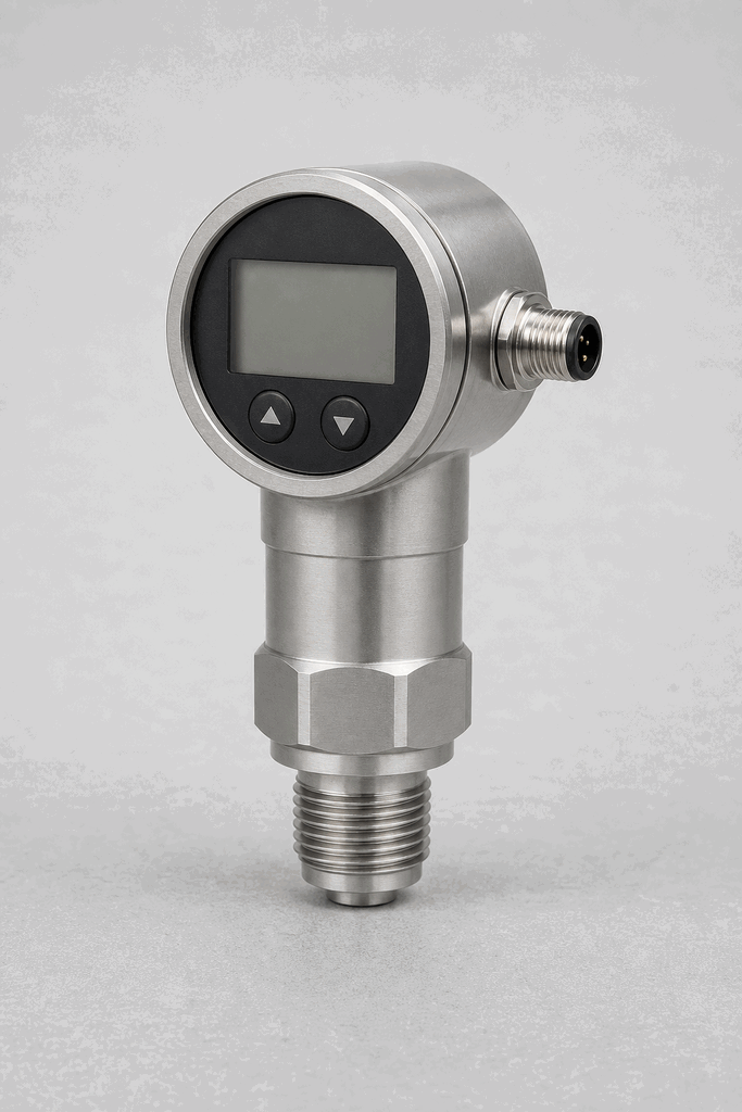
Representative real-world Pressure Transmitter (4-20 mA) hardware on an industrial workbench
Representative field appearance · form factors vary by manufacturer

Hardware recognition

Know what to look for

Use the silhouette, active face, and connection style to identify the device before checking its part number and datasheet.

Body and mounting
A stainless process fitting supports a cylindrical or rectangular electronic head.
Active face
The wetted diaphragm sits behind the threaded or hygienic process connection.
Cable and terminals
An M12 plug, DIN connector, or cable carries the 4–20 mA loop.
Field rule: identify by appearance, then verify the exact wiring, range, approvals, and output type from the device label and datasheet.

02 / Understand the principle

Watch cause become a PLC signal

Follow the physical event through the sensing element and into the exact controller value.

Signal story / live loop

Pressure Transmitter (4-20 mA): cause to controller

Paused

Now showingPhysical event

Line pressure rises → Diaphragm deflects → %IW64 = 19,354

03 / Test and commission it

Commission it on the bench

Move the process, adjust the setpoint, invert the logic and inject faults. Watch the PLC value respond immediately.

Commissioning bench

Pressure Transmitter (4-20 mA)

24 VDC%IW64
9.60 mA
3.5 bar
7 bar

PLC channel

%IW64

RAW 9677

Engineering value

3.5 bar

Loop current

Output logic
Inject a field fault

Channel healthy

Signal is inside the expected operating range

Terminals
+24 V4–20 mA loop +AI− / 0 V

Commissioning note: Confirm the transmitter range and PLC scaling use the same engineering units.

Field guide

A pressure transmitter measures process pressure and converts it to a 4-20 milliamp current signal. At the minimum process pressure (0 bar, or whatever the lower range value is), the transmitter outputs exactly 4 mA. At the maximum (e.g. 10 bar), it outputs 20 mA. The current is proportional to the pressure anywhere between those extremes.

The 4-20 mA current loop is the industry standard for analog field devices because current is far more noise-immune than voltage over long cable runs. A voltage signal loses amplitude with cable resistance; a current source drives through the same resistance without losing signal integrity.

The 4 mA live zero is safety-relevant: if the signal falls below 4 mA the PLC knows the cable is broken or the transmitter has lost power — zero mA is not a valid process reading, it is a wire-fault. This lets the control system take protective action rather than treating a fault as "minimum pressure".

PLC analog input cards convert the current to a raw integer count (typically 0-27648 on Siemens, 6241-31208 for 4-20 mA on Allen-Bradley). A scaling block (FC105 in Siemens STEP 7, SCL in Studio 5000) converts the raw count to engineering units: bars, PSI, or kPa.

The internal sensing element is usually a piezo-resistive bridge or a ceramic capacitive cell. Both change their electrical properties under mechanical deformation caused by pressure, and the transmitter electronics condition this tiny signal into the standard current output.

Use this when…

  • Monitoring pipeline pressure in a water or compressed-air system
  • Providing feedback for a PID pressure control loop
  • Detecting a blocked filter or pump cavitation via differential pressure

Where you will see it

HVAC

Differential pressure transmitters across air-handling units control variable-speed drives on fans, keeping static pressure constant.

Oil and gas

Pressure transmitters on wellheads and separators give the SCADA system real-time process data for safety shut-down logic.

PLC wiring reference

Trace the complete electrical path instead of treating the PLC tag as magic. Confirm the device datasheet before wiring real hardware.

  1. 1+24 V
  2. 24–20 mA loop +
  3. 3AI− / 0 V

Commissioning checkpoint

Confirm the transmitter range and PLC scaling use the same engineering units.

PLC address
%IW64
Expected signal
Loop current

Field questions

Frequently asked questions

What signal does a Pressure Transmitter (4-20 mA) send to a PLC?

Loop current is read at %IW64. The exact electrical connection is +24 V, 4–20 mA loop +, AI− / 0 V.

How do you commission a Pressure Transmitter (4-20 mA)?

Confirm the transmitter range and PLC scaling use the same engineering units.

Next skill

Connect it to PLC logic

Unlock PLC integration challenges

See plans

Free first success

Use the pressure transmitter (4-20 ma) signal in PLC logic

Apply the wiring and commissioning model in a scored browser exercise, then save your progress and continue through the recommended path.

No installNo credit cardImmediate pass/fail feedback

Technical reference and worked-example guide

Pressure transmitter PLC guide: implementation, evidence and troubleshooting

Direct answer

Pressure transmitter PLC guide becomes useful when it connects pressure type, reference, range, span, units, overpressure, wetted materials, process connection, impulse line, damping, output standard, loop supply, accuracy and failure indication with process pressure through connection and sensing element to transmitter output, loop, plc input, raw conversion, scaled value, quality, alarm and control decision, then proves zero, midpoint and high reference conditions produce stable engineering values within the declared system tolerance under normal, boundary, fault and recovery conditions. The objective is a repeatable engineering or learning result, not merely activity inside a page or tool.

This guide is written for instrumentation and PLC learners connecting gauge, absolute or differential pressure transmitters to analog inputs. The intended result is specific: the reader can specify pressure reference and units, trace the electrical loop, scale raw values and distinguish process, impulse-line, transmitter, wiring and input faults.

an instrumentation calibration bench connecting pressure, temperature, load, level and smart sensors to PLC input channels and reference measurements while studying pressure transmitter range, loop, scaling and diagnostic evidence
The scene connects pressure transmitter range, loop, scaling and diagnostic evidence to declared conditions, safe boundaries, observable evidence and a repeatable result.

System map / 02

Six concepts that control the result

Treat these as connected checkpoints. Each checkpoint has an expected state, an observable state and a boundary to the next part of the system. That structure prevents a software indication from being mistaken for physical proof.

NODE 01observable

Define the operating contract

pressure type, reference, range, span, units, overpressure, wetted materials, process connection, impulse line, damping, output standard, loop supply, accuracy and failure indication. For pressure transmitter range, loop, scaling and diagnostic evidence, record the initial condition, actor, requested change, observable result and stopping condition before selecting a tool or implementation.

NODE 02observable

Map the evidence path

process pressure through connection and sensing element to transmitter output, loop, PLC input, raw conversion, scaled value, quality, alarm and control decision. Separate request, internal state, output or service, physical or user-visible result and independent feedback so each boundary can be inspected.

NODE 03observable

Prove normal operation

zero, midpoint and high reference conditions produce stable engineering values within the declared system tolerance. Run more than one cycle from a known state and retain the values, timings or artifacts that demonstrate repeatability.

NODE 04observable

Exercise a boundary case

blocked or leaking impulse line, overrange, reversed manifold, lost loop power, open circuit, wrong input mode, offset, drift, damping and restart. Choose minimum, maximum, simultaneous, delayed or restart conditions that reveal assumptions hidden by the happy path.

NODE 05observable

Diagnose a controlled fault

a process, reference, connection, transmitter, supply, wiring, input, conversion, scale or unit mismatch. Preserve the first symptom, divide the system at a measurable boundary and change one condition only after predicting the result.

NODE 06observable

Transfer and hand over

the installation inspected and calibrated with approved pressure references and procedures. Restore normal state, remove temporary changes, repeat affected checks and document which claims remain limited to the learning environment.

Procedure / 03

A six-step practice and commissioning workflow

Run the steps in order the first time. Later, the same structure becomes a diagnostic loop: define the expected condition, observe the boundary, interpret the difference and choose one proving action.

  1. 01

    Write the acceptance case

    Convert pressure type, reference, range, span, units, overpressure, wetted materials, process connection, impulse line, damping, output standard, loop supply, accuracy and failure indication into initial conditions, one stimulus and observable pass criteria.

    Evidence: Another person can repeat the case without guessing the intended result.

    Avoid: Using page completion or an animation as the acceptance criterion.

  2. 02

    Build the map

    Document process pressure through connection and sensing element to transmitter output, loop, plc input, raw conversion, scaled value, quality, alarm and control decision and name who owns each state or decision.

    Evidence: Every request and result has a source, destination and useful inspection point.

    Avoid: Using the same value as command, status and independent feedback.

  3. 03

    Run the baseline

    Apply zero, midpoint and high reference conditions produce stable engineering values within the declared system tolerance from a clean start and record the expected evidence.

    Evidence: Repeated runs produce the same bounded result.

    Avoid: Changing several parameters before a baseline exists.

  4. 04

    Challenge assumptions

    Test blocked or leaking impulse line, overrange, reversed manifold, lost loop power, open circuit, wrong input mode, offset, drift, damping and restart without changing the acceptance contract.

    Evidence: Limits, timing and restart behavior reach defined states.

    Avoid: Testing only one ideal sequence.

  5. 05

    Isolate one failure

    Introduce or analyse a process, reference, connection, transmitter, supply, wiring, input, conversion, scale or unit mismatch and locate the first disagreement.

    Evidence: The proving action distinguishes the leading hypotheses.

    Avoid: Resetting, forcing or replacing before evidence is retained.

  6. 06

    Close the evidence loop

    Complete the installation inspected and calibrated with approved pressure references and procedures and repeat the affected regression cases.

    Evidence: Reference use is complete when inputs, assumptions, units or initial conditions are recorded and the result is independently checked at a useful boundary.

    Avoid: Treating an acknowledged message or one successful rerun as handover.

Diagnostic matrix / 04

Symptoms, proving points and next actions

The table is a reasoning aid, not a parts-replacement chart. Preserve the initial symptom, inspect the named boundary and use the interpretation to choose the next controlled test. Site safety procedures and equipment manuals remain authoritative.

Diagnostic symptoms, inspection points, interpretations and next actions for Pressure transmitter PLC guide: implementation, evidence and troubleshooting
Observed symptomInspectInterpretationNext proving action
The expected result is unclearRequirement, initial state, actor, stimulus, units and pass conditionThe technician, programmer and reviewer may be solving different versions of the task.Rewrite one observable acceptance case before continuing.
Internal state changes but the outcome does notRequest, final owner, output or service boundary and independent feedbackA software or interface indication proves intent at one layer, not the complete outcome.Trace the first boundary after the changing state.
Normal case passes but an edge case failsLimits, timing, simultaneous events, reset and restart assumptionsThe implementation contains a hidden assumption exposed by the changed condition.Add the failed boundary as a permanent regression case.
The failure disappears after resetOriginal symptom, histories, diagnostics, timestamps and active causeReset changed evidence or state without proving the initiating cause.Reproduce under a controlled condition and preserve pre/post-event data.
Simulator and target disagreeModel boundary, software version, task timing, I/O behavior, data types and configurationA learning model and the intended target do not share one of the recorded assumptions.Reduce the case and verify against current target documentation.
The result cannot be explainedPrediction, observation, proving action, alternative hypotheses and limitationsActivity occurred but the evidence is not yet transferable or reviewable.Have the learner defend the signal path and repeat a changed case.

Product evidence / 05

What the browser practice can actually demonstrate

The page connects definitions and worked examples to runnable tools, explicit assumptions and repeatable checks so a formula or pattern can be challenged.

Where simulation stops

A generic guide cannot select pressure rating, wetted materials, hazardous-area protection or calibration method; current process and device requirements govern.

Commissioning notebook / 06

Six cases that turn the concepts into evidence

Use these as written briefs rather than click-through instructions. For every case, state the expected condition before acting, retain the first useful observation and explain why the final result proves the requirement. A different program or component choice can still be correct when it produces the same bounded behavior and evidence.

Case 01

predict → observe → prove

Prove define the operating contract

Engineering context. pressure type, reference, range, span, units, overpressure, wetted materials, process connection, impulse line, damping, output standard, loop supply, accuracy and failure indication. For pressure transmitter range, loop, scaling and diagnostic evidence, record the initial condition, actor, requested change, observable result and stopping condition before selecting a tool or implementation. Begin with a written normal condition and identify which request, state, physical result or communication value will provide independent confirmation. Do not begin by changing the configuration; the initial state is part of the evidence and should remain reproducible.

Controlled setup. Use the “Write the acceptance case” stage of the workflow: convert pressure type, reference, range, span, units, overpressure, wetted materials, process connection, impulse line, damping, output standard, loop supply, accuracy and failure indication into initial conditions, one stimulus and observable pass criteria. The acceptance record should show this result: another person can repeat the case without guessing the intended result. Record initial conditions, the exact stimulus and the observation point so another learner can repeat the case without relying on your memory.

Fault challenge. Introduce or analyse “The expected result is unclear” as one bounded deviation. Inspect requirement, initial state, actor, stimulus, units and pass condition The working interpretation is that the technician, programmer and reviewer may be solving different versions of the task. The next proving action is to rewrite one observable acceptance case before continuing. Change only one condition before observing the result, and preserve timestamps or measurements where timing matters.

Review and recovery. The most common trap here is using page completion or an animation as the acceptance criterion. After restoring the cause, repeat the normal case and at least one stop, timeout, disconnect or restart boundary relevant to this topic. Remove temporary forces and bypasses, return the model to a known state and retain the evidence that both operation and recovery are deliberate.

Explain it aloud: How is a pressure transmitter connected to a PLC? A defensible short answer is: Connect its compatible current, voltage or digital output through the complete supply and return path to the configured input, then scale the declared range and units.

Case 02

predict → observe → prove

Prove map the evidence path

Engineering context. process pressure through connection and sensing element to transmitter output, loop, PLC input, raw conversion, scaled value, quality, alarm and control decision. Separate request, internal state, output or service, physical or user-visible result and independent feedback so each boundary can be inspected. Begin with a written normal condition and identify which request, state, physical result or communication value will provide independent confirmation. Do not begin by changing the configuration; the initial state is part of the evidence and should remain reproducible.

Controlled setup. Use the “Build the map” stage of the workflow: document process pressure through connection and sensing element to transmitter output, loop, plc input, raw conversion, scaled value, quality, alarm and control decision and name who owns each state or decision. The acceptance record should show this result: every request and result has a source, destination and useful inspection point. Record initial conditions, the exact stimulus and the observation point so another learner can repeat the case without relying on your memory.

Fault challenge. Introduce or analyse “Internal state changes but the outcome does not” as one bounded deviation. Inspect request, final owner, output or service boundary and independent feedback The working interpretation is that a software or interface indication proves intent at one layer, not the complete outcome. The next proving action is to trace the first boundary after the changing state. Change only one condition before observing the result, and preserve timestamps or measurements where timing matters.

Review and recovery. The most common trap here is using the same value as command, status and independent feedback. After restoring the cause, repeat the normal case and at least one stop, timeout, disconnect or restart boundary relevant to this topic. Remove temporary forces and bypasses, return the model to a known state and retain the evidence that both operation and recovery are deliberate.

Explain it aloud: What is the difference between gauge and absolute pressure? A defensible short answer is: Gauge pressure is referenced to local atmospheric pressure, while absolute pressure is referenced to a vacuum; the selected reference changes the engineering meaning.

Case 03

predict → observe → prove

Prove prove normal operation

Engineering context. zero, midpoint and high reference conditions produce stable engineering values within the declared system tolerance. Run more than one cycle from a known state and retain the values, timings or artifacts that demonstrate repeatability. Begin with a written normal condition and identify which request, state, physical result or communication value will provide independent confirmation. Do not begin by changing the configuration; the initial state is part of the evidence and should remain reproducible.

Controlled setup. Use the “Run the baseline” stage of the workflow: apply zero, midpoint and high reference conditions produce stable engineering values within the declared system tolerance from a clean start and record the expected evidence. The acceptance record should show this result: repeated runs produce the same bounded result. Record initial conditions, the exact stimulus and the observation point so another learner can repeat the case without relying on your memory.

Fault challenge. Introduce or analyse “Normal case passes but an edge case fails” as one bounded deviation. Inspect limits, timing, simultaneous events, reset and restart assumptions The working interpretation is that the implementation contains a hidden assumption exposed by the changed condition. The next proving action is to add the failed boundary as a permanent regression case. Change only one condition before observing the result, and preserve timestamps or measurements where timing matters.

Review and recovery. The most common trap here is changing several parameters before a baseline exists. After restoring the cause, repeat the normal case and at least one stop, timeout, disconnect or restart boundary relevant to this topic. Remove temporary forces and bypasses, return the model to a known state and retain the evidence that both operation and recovery are deliberate.

Explain it aloud: What should I learn first about pressure transmitter range, loop, scaling and diagnostic evidence? A defensible short answer is: Start with the operating contract and evidence path: pressure type, reference, range, span, units, overpressure, wetted materials, process connection, impulse line, damping, output standard, loop supply, accuracy and failure indication, followed by process pressure through connection and sensing element to transmitter output, loop, plc input, raw conversion, scaled value, quality, alarm and control decision. Add advanced features only after the baseline is predictable.

Case 04

predict → observe → prove

Prove exercise a boundary case

Engineering context. blocked or leaking impulse line, overrange, reversed manifold, lost loop power, open circuit, wrong input mode, offset, drift, damping and restart. Choose minimum, maximum, simultaneous, delayed or restart conditions that reveal assumptions hidden by the happy path. Begin with a written normal condition and identify which request, state, physical result or communication value will provide independent confirmation. Do not begin by changing the configuration; the initial state is part of the evidence and should remain reproducible.

Controlled setup. Use the “Challenge assumptions” stage of the workflow: test blocked or leaking impulse line, overrange, reversed manifold, lost loop power, open circuit, wrong input mode, offset, drift, damping and restart without changing the acceptance contract. The acceptance record should show this result: limits, timing and restart behavior reach defined states. Record initial conditions, the exact stimulus and the observation point so another learner can repeat the case without relying on your memory.

Fault challenge. Introduce or analyse “The failure disappears after reset” as one bounded deviation. Inspect original symptom, histories, diagnostics, timestamps and active cause The working interpretation is that reset changed evidence or state without proving the initiating cause. The next proving action is to reproduce under a controlled condition and preserve pre/post-event data. Change only one condition before observing the result, and preserve timestamps or measurements where timing matters.

Review and recovery. The most common trap here is testing only one ideal sequence. After restoring the cause, repeat the normal case and at least one stop, timeout, disconnect or restart boundary relevant to this topic. Remove temporary forces and bypasses, return the model to a known state and retain the evidence that both operation and recovery are deliberate.

Explain it aloud: How do I practise pressure transmitter range, loop, scaling and diagnostic evidence effectively? A defensible short answer is: Use short cases with known initial conditions, a written prediction, one action and an observable result. Then alter a boundary or fault and explain why the evidence changed.

Case 05

predict → observe → prove

Prove diagnose a controlled fault

Engineering context. a process, reference, connection, transmitter, supply, wiring, input, conversion, scale or unit mismatch. Preserve the first symptom, divide the system at a measurable boundary and change one condition only after predicting the result. Begin with a written normal condition and identify which request, state, physical result or communication value will provide independent confirmation. Do not begin by changing the configuration; the initial state is part of the evidence and should remain reproducible.

Controlled setup. Use the “Isolate one failure” stage of the workflow: introduce or analyse a process, reference, connection, transmitter, supply, wiring, input, conversion, scale or unit mismatch and locate the first disagreement. The acceptance record should show this result: the proving action distinguishes the leading hypotheses. Record initial conditions, the exact stimulus and the observation point so another learner can repeat the case without relying on your memory.

Fault challenge. Introduce or analyse “Simulator and target disagree” as one bounded deviation. Inspect model boundary, software version, task timing, I/O behavior, data types and configuration The working interpretation is that a learning model and the intended target do not share one of the recorded assumptions. The next proving action is to reduce the case and verify against current target documentation. Change only one condition before observing the result, and preserve timestamps or measurements where timing matters.

Review and recovery. The most common trap here is resetting, forcing or replacing before evidence is retained. After restoring the cause, repeat the normal case and at least one stop, timeout, disconnect or restart boundary relevant to this topic. Remove temporary forces and bypasses, return the model to a known state and retain the evidence that both operation and recovery are deliberate.

Explain it aloud: What counts as proof of competence? A defensible short answer is: A repeatable artifact or system result plus an explanation of the signal path is stronger than time spent, screenshots or a copied answer. Physical competence requires separate supervised evidence.

Case 06

predict → observe → prove

Prove transfer and hand over

Engineering context. the installation inspected and calibrated with approved pressure references and procedures. Restore normal state, remove temporary changes, repeat affected checks and document which claims remain limited to the learning environment. Begin with a written normal condition and identify which request, state, physical result or communication value will provide independent confirmation. Do not begin by changing the configuration; the initial state is part of the evidence and should remain reproducible.

Controlled setup. Use the “Close the evidence loop” stage of the workflow: complete the installation inspected and calibrated with approved pressure references and procedures and repeat the affected regression cases. The acceptance record should show this result: reference use is complete when inputs, assumptions, units or initial conditions are recorded and the result is independently checked at a useful boundary. Record initial conditions, the exact stimulus and the observation point so another learner can repeat the case without relying on your memory.

Fault challenge. Introduce or analyse “The result cannot be explained” as one bounded deviation. Inspect prediction, observation, proving action, alternative hypotheses and limitations The working interpretation is that activity occurred but the evidence is not yet transferable or reviewable. The next proving action is to have the learner defend the signal path and repeat a changed case. Change only one condition before observing the result, and preserve timestamps or measurements where timing matters.

Review and recovery. The most common trap here is treating an acknowledged message or one successful rerun as handover. After restoring the cause, repeat the normal case and at least one stop, timeout, disconnect or restart boundary relevant to this topic. Remove temporary forces and bypasses, return the model to a known state and retain the evidence that both operation and recovery are deliberate.

Explain it aloud: Why test faults and restart behavior? A defensible short answer is: Because a process, reference, connection, transmitter, supply, wiring, input, conversion, scale or unit mismatch or blocked or leaking impulse line, overrange, reversed manifold, lost loop power, open circuit, wrong input mode, offset, drift, damping and restart can expose assumptions that never appear during ideal startup and steady operation.

Answer surface / 07

Questions people ask about Pressure transmitter PLC guide

These concise answers define the operating, training and product boundaries most often missed in broad summaries. The full workflow and diagnostic table above provide the evidence behind them.

How is a pressure transmitter connected to a PLC?

Connect its compatible current, voltage or digital output through the complete supply and return path to the configured input, then scale the declared range and units.

What is the difference between gauge and absolute pressure?

Gauge pressure is referenced to local atmospheric pressure, while absolute pressure is referenced to a vacuum; the selected reference changes the engineering meaning.

What should I learn first about pressure transmitter range, loop, scaling and diagnostic evidence?

Start with the operating contract and evidence path: pressure type, reference, range, span, units, overpressure, wetted materials, process connection, impulse line, damping, output standard, loop supply, accuracy and failure indication, followed by process pressure through connection and sensing element to transmitter output, loop, plc input, raw conversion, scaled value, quality, alarm and control decision. Add advanced features only after the baseline is predictable.

How do I practise pressure transmitter range, loop, scaling and diagnostic evidence effectively?

Use short cases with known initial conditions, a written prediction, one action and an observable result. Then alter a boundary or fault and explain why the evidence changed.

What counts as proof of competence?

A repeatable artifact or system result plus an explanation of the signal path is stronger than time spent, screenshots or a copied answer. Physical competence requires separate supervised evidence.

Why test faults and restart behavior?

Because a process, reference, connection, transmitter, supply, wiring, input, conversion, scale or unit mismatch or blocked or leaking impulse line, overrange, reversed manifold, lost loop power, open circuit, wrong input mode, offset, drift, damping and restart can expose assumptions that never appear during ideal startup and steady operation.

Can browser practice replace official software or hardware?

No. It can build concepts and diagnostic reasoning. Exact firmware, I/O electrical behavior, networking, safety and commissioning require current official tools, documentation and target equipment.

How should progress be documented?

Keep the requirement, initial state, program or configuration, observed values, fault hypothesis, proving action, recovery result and a concise limitations statement.

Real 4-20ma pressure transmitter footage

See this exact skill in the working simulator.

Watch the real browser product respond to the task on this page, then try the same practical workflow yourself. No slides, concept mockups, install, or credit card.

Try this in the browser
4–20 mA Pressure Transmitter — Signal, Scaling and Faults