Skip to learning content
Field instrumentation lab

Understand the signal. Commission the device. Diagnose the fault.

Animated industrial sensors with live setpoints, PLC values, wiring terminals and realistic failure modes—built for technicians, controls engineers and apprentices.

No install. No credit card. Start with a visible result.
17device labs
4–20mA scaling
3fault modes
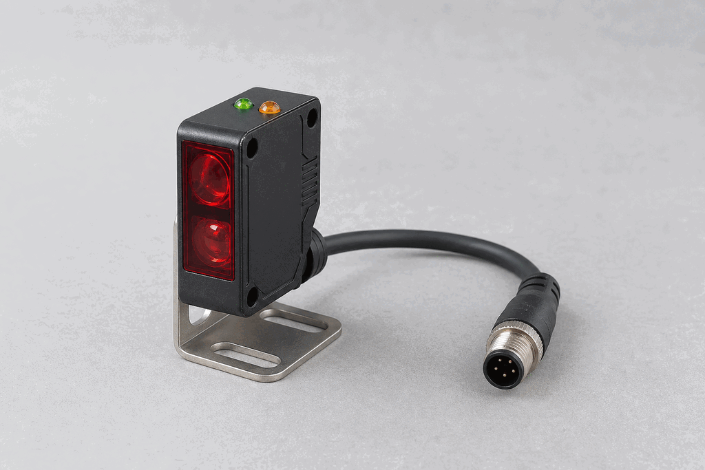
Real industrial photoelectric sensor with dual optical lenses, mounting bracket and M12 connector
Real field device
INPUT %I0.0 ONSUPPLY 24.1 VSTATUS HEALTHY

Choose a bench

Industrial sensor catalogue

Start with a physical device, then trace its signal into the PLC.

Showing 17 of 17 labs
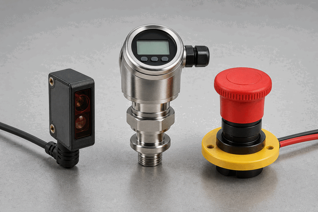
Representative field hardware: Industrial Sensors — A First LookLab 01Field hardware
Discrete inputFoundation

Industrial Sensors — A First Look

Meet the three sensor families — discrete, analog, and safety — and learn which one your application needs.

Live workbenchOpen lab
Representative field hardware: Photoelectric Sensor (Photoeye)Lab 02Field hardware
Discrete inputFoundation

Photoelectric Sensor (Photoeye)

Detects parts as they pass — outputs a discrete bit when something blocks the light beam.
Live workbenchOpen lab
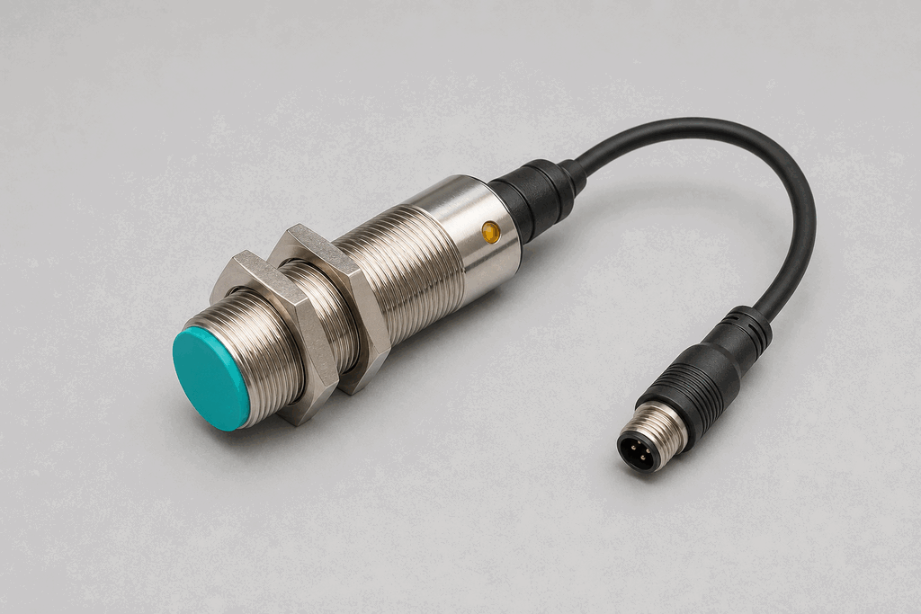
Representative field hardware: Inductive Proximity SensorLab 03Field hardware
Discrete inputFoundation

Inductive Proximity Sensor

Detects metallic targets without contact by sensing changes in an electromagnetic field.
Live workbenchOpen lab
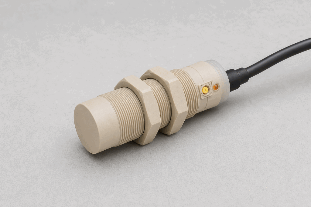
Representative field hardware: Capacitive Proximity SensorLab 04Field hardware
Discrete inputFoundation

Capacitive Proximity Sensor

Detects any material — metal, plastic, liquid, or granular — by sensing the change in capacitance at the sensing face.
Live workbenchOpen lab
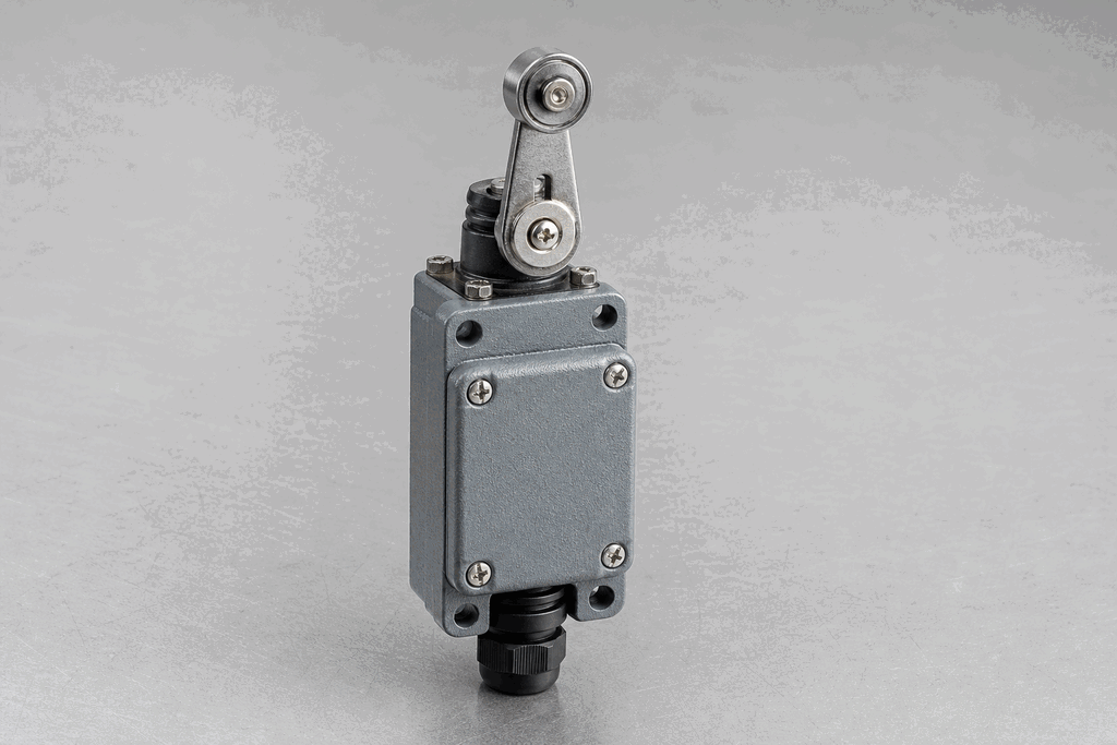
Representative field hardware: Mechanical Limit SwitchLab 05Field hardware
Discrete inputFoundation

Mechanical Limit Switch

A mechanical contact switch that changes state when a moving part physically depresses its actuator.
Live workbenchOpen lab
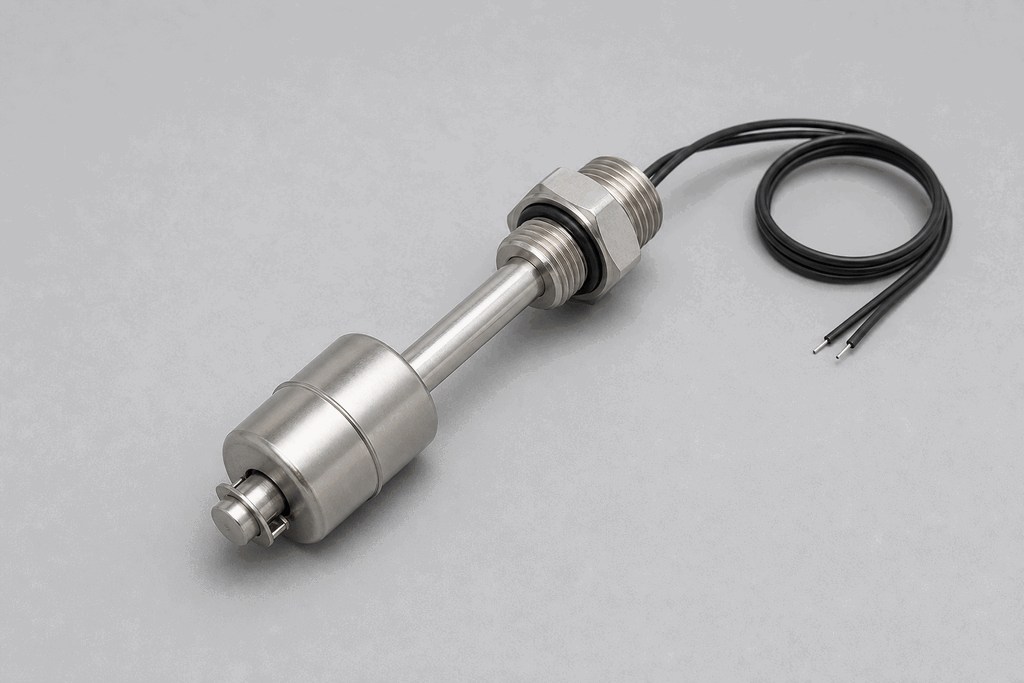
Representative field hardware: Float Switch (Level Switch)Lab 06Field hardware
Discrete inputField practice

Float Switch (Level Switch)

A buoyancy-driven switch that opens or closes when liquid level rises to or falls from a set point.
Live workbenchOpen lab
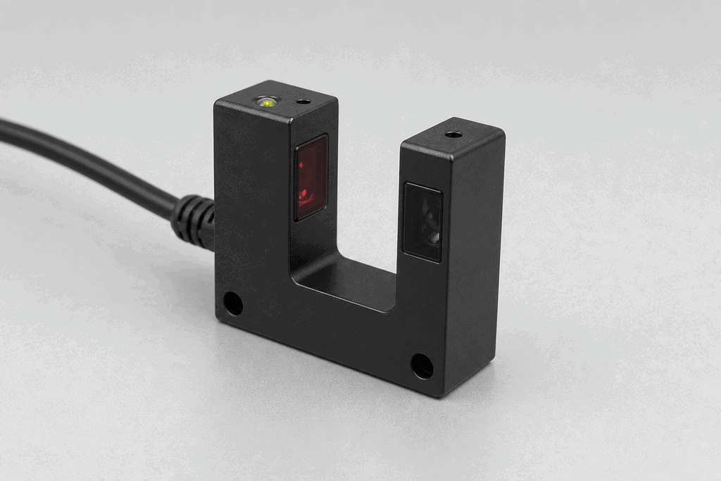
Representative field hardware: Photo-Fork Sensor (Slot Sensor)Lab 07Field hardware
Discrete inputField practice

Photo-Fork Sensor (Slot Sensor)

A U-shaped optical sensor with emitter and receiver built into opposite tines — detects objects passing through the gap.
Live workbenchOpen lab
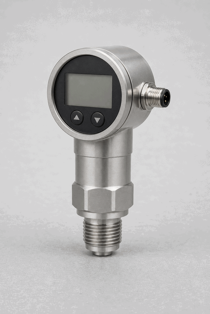
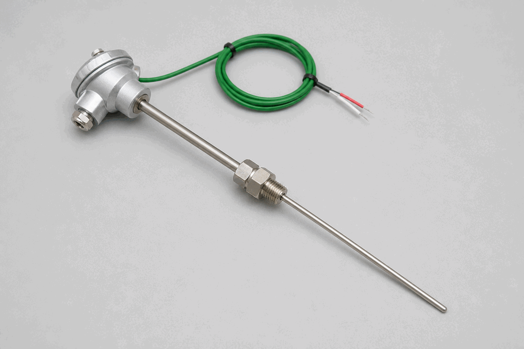
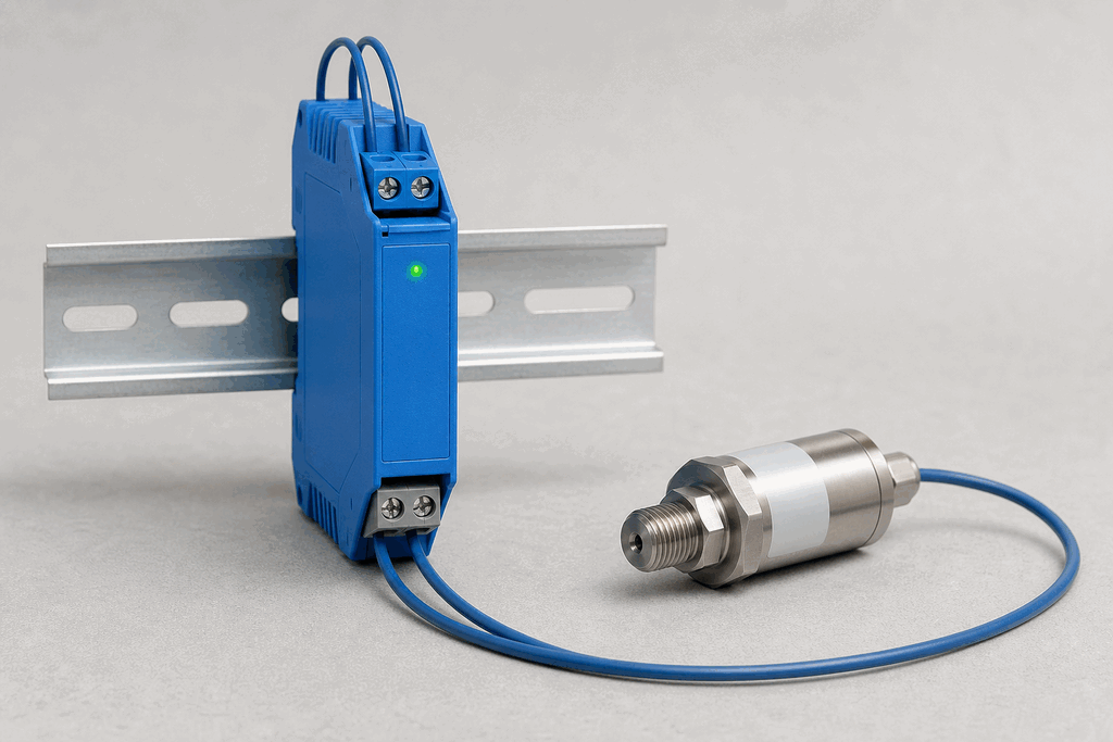
Representative field hardware: Pressure Transmitter (4-20 mA)Lab 08Field hardware
Analog inputField practice

Pressure Transmitter (4-20 mA)

Converts process pressure to a 4-20 mA current loop signal proportional to the engineering-unit range.
Live workbenchOpen lab
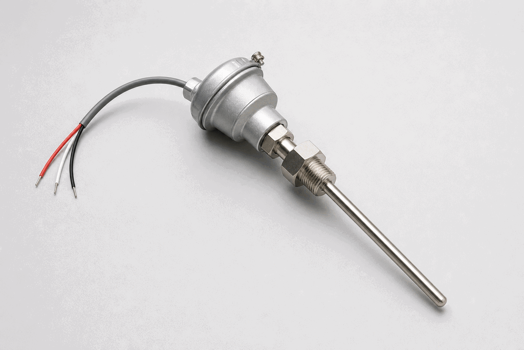
Representative field hardware: Thermocouple (Type K)Lab 09Field hardware
Analog inputField practice

Thermocouple (Type K)

Two dissimilar metal wires joined at a measurement junction produce a millivolt signal proportional to temperature.
Live workbenchOpen lab
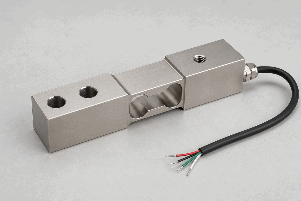
Representative field hardware: RTD / PT100 Temperature SensorLab 10Field hardware
Analog inputField practice

RTD / PT100 Temperature Sensor

A platinum resistance thermometer whose resistance increases linearly with temperature — more accurate and more stable than a thermocouple over the 0–500 °C industrial range.
Live workbenchOpen lab
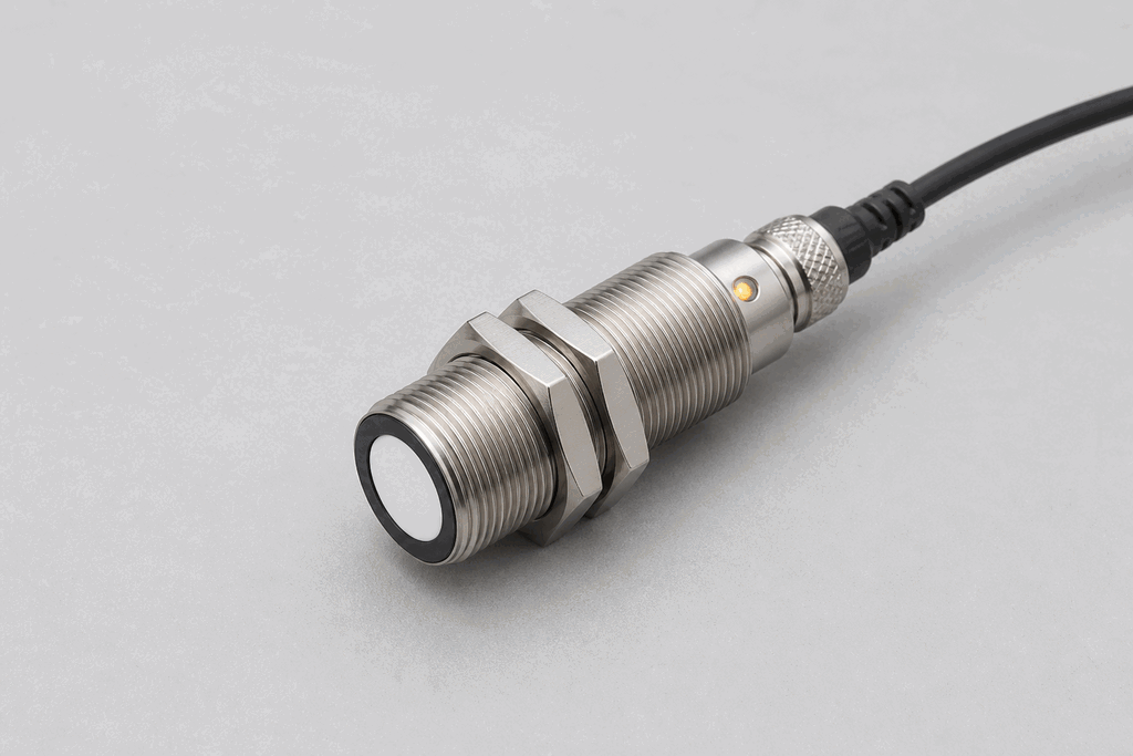
Representative field hardware: Strain Gauge / Load CellLab 11Field hardware
Analog inputAdvanced

Strain Gauge / Load Cell

Measures mechanical force or weight by detecting tiny resistance changes in metal foil bonded to a structural element.
Live workbenchOpen lab
Representative field hardware: Ultrasonic Distance SensorLab 12Field hardware
Analog inputField practice

Ultrasonic Distance Sensor

Measures distance by timing an ultrasonic pulse echo — output is proportional to the target distance.
Live workbenchOpen lab
Representative field hardware: Incremental Encoder (Quadrature)Lab 13Field hardware
Analog inputField practice

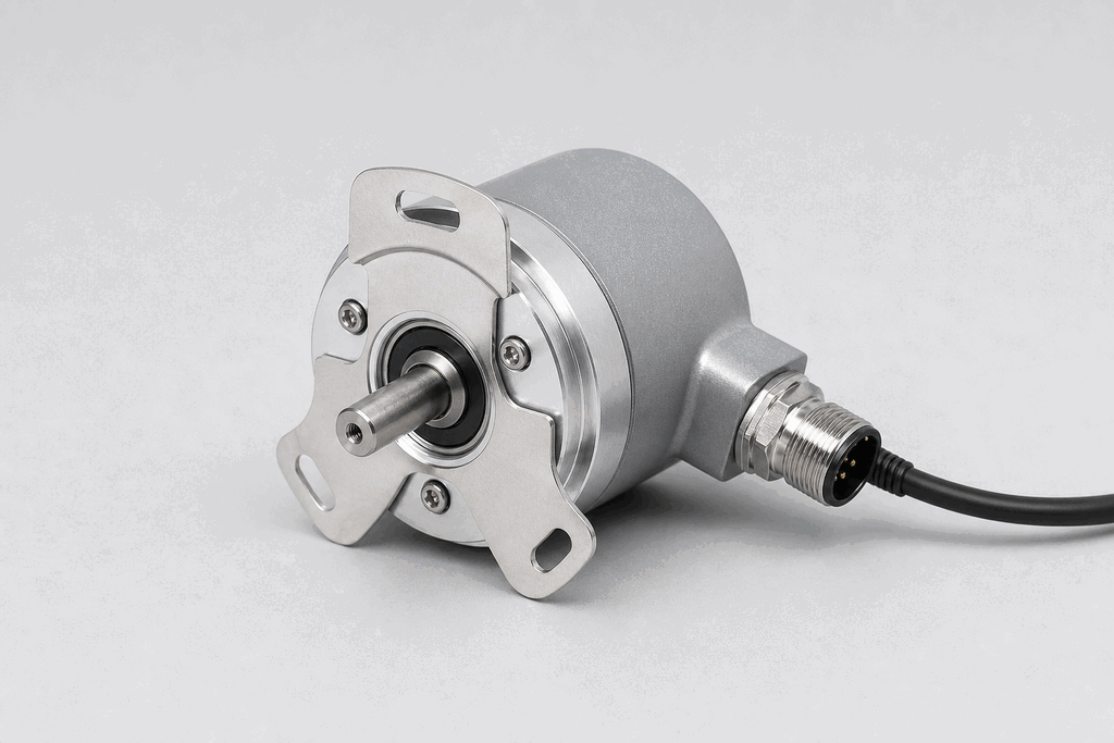
Incremental Encoder (Quadrature)

Converts shaft rotation into a pulse train — two channels (A and B) in quadrature give position and direction.
Live workbenchOpen lab
Representative field hardware: Safety Light CurtainLab 14Field hardware
Safety inputAdvanced

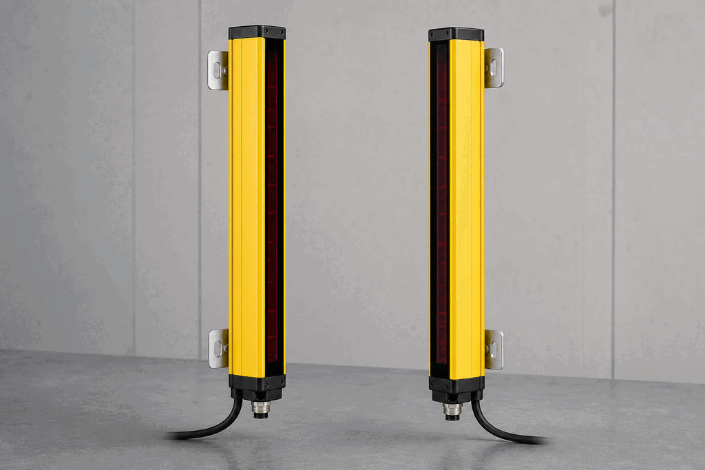
Safety Light Curtain

An optical safety device forming a grid of infrared beams — breaking any beam immediately stops hazardous machine motion.
Live workbenchOpen lab
Representative field hardware: E-Stop Circuit (Cat 3 / Cat 4)Lab 15Field hardware
Safety inputAdvanced

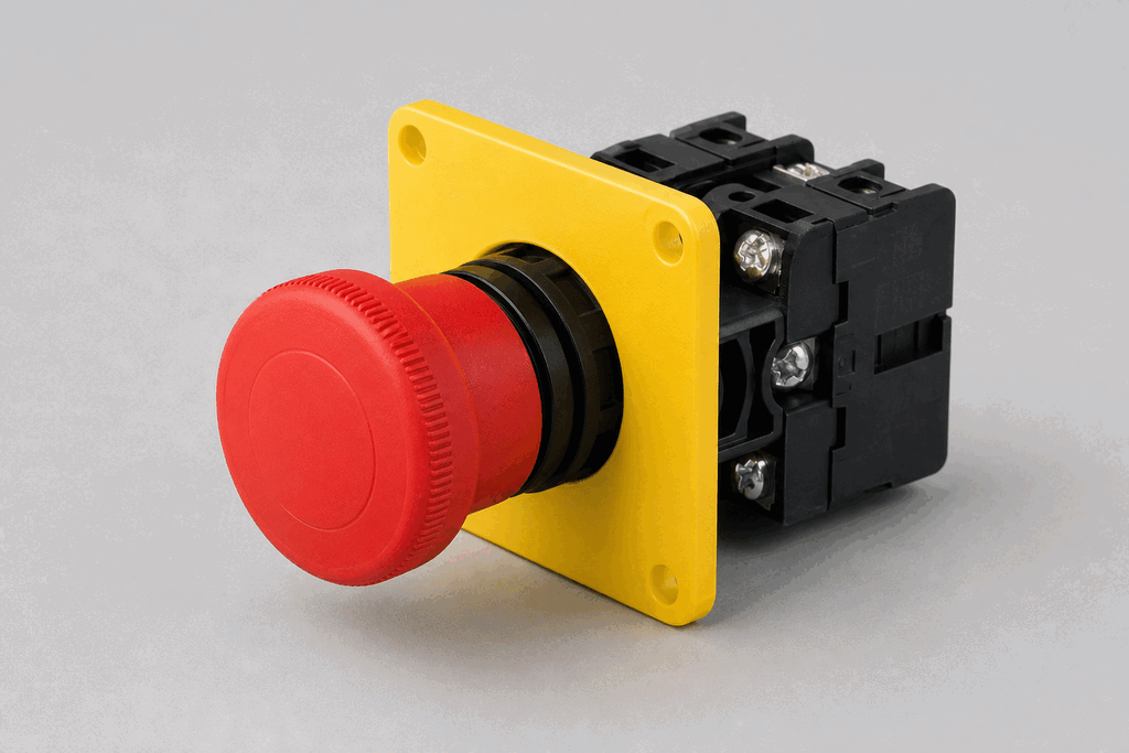
E-Stop Circuit (Cat 3 / Cat 4)

A dual-channel monitored emergency stop circuit that safely removes power from hazardous motion and detects single-point failures.
Live workbenchOpen lab
Representative field hardware: IO-Link Smart SensorsLab 16Field hardware
Discrete inputAdvanced

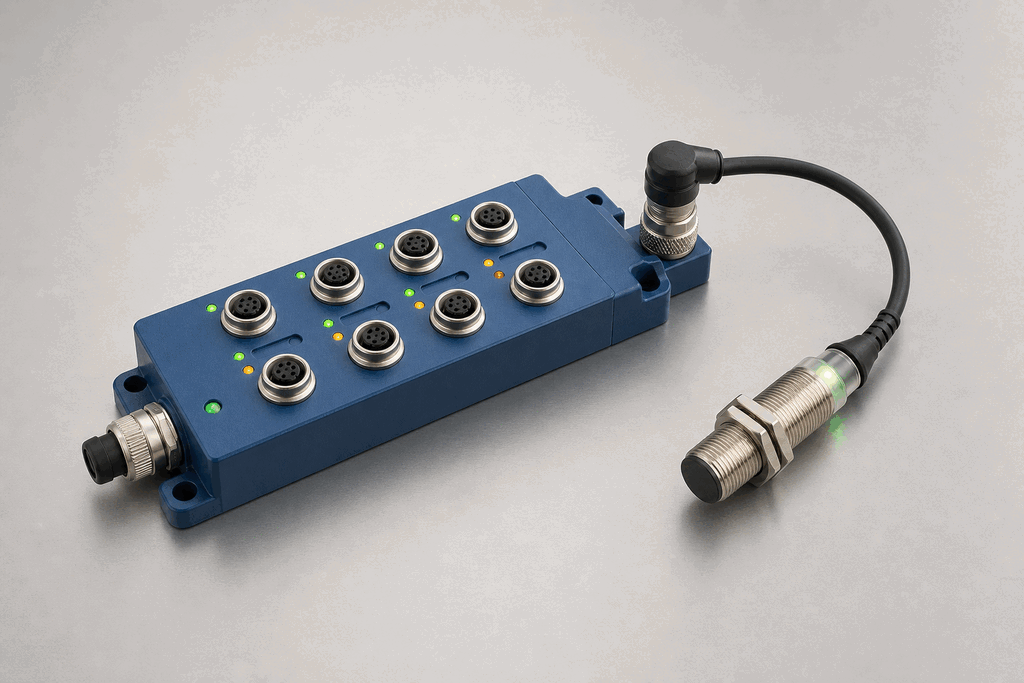
IO-Link Smart Sensors

IO-Link turns an ordinary point-to-point sensor cable into a bidirectional digital channel — unlocking remote parameterisation, rich diagnostics, and event data alongside the normal process value.
Live workbenchOpen lab
Representative field hardware: Intrinsic Safety in Hazardous AreasLab 17Field hardware
Safety inputAdvanced

Intrinsic Safety in Hazardous Areas

Intrinsically safe sensors limit the electrical energy in a hazardous area circuit so that no ignition-capable spark or hot surface can form — even under fault conditions. Zener barriers and galvanic isolators enforce the energy limits between the safe zone and the explosive atmosphere.

Live workbenchOpen lab

From field condition to PLC value

Choose the signal family before the device

Discrete detection

Use a photoeye, proximity sensor or limit switch when the controller needs a reliable yes/no state such as part present or guard closed.

Analog measurement

Use a transmitter, temperature element or load cell when the PLC must scale a changing physical value into engineering units.

Safety detection

Use validated safety devices and safety logic when a detection failure could expose a person to hazardous motion. A standard input alone is not a safety function.

Free first success

Wire the signal into a real PLC decision

Use a guided browser lab to see an input change, run the logic and get immediate feedback before creating a free account to save the result.

No installNo credit cardImmediate pass/fail feedback

Industrial sensor selection field guide

Industrial sensors for PLCs: selection, wiring and fault evidence

Direct answer

Choose an industrial sensor from the physical variable, target, environment, response time, range, output type, wiring interface and failure behavior. Commission it by proving the physical change at the device, module channel and PLC tag—not by trusting one indicator.

This guide is written for pLC learners, maintenance technicians, panel builders and controls engineers comparing discrete, analog, position and safety-related sensing methods. The intended result is specific: the learner can select the sensing principle, identify the electrical contract, map the signal to a PLC and diagnose the first disagreement between physical target and program value.

System map / 02

Six concepts that control the result

Treat these as connected checkpoints. Each checkpoint has an expected state, an observable state and a boundary to the next part of the system. That structure prevents a software indication from being mistaken for physical proof.

NODE 01observable

Measured variable

Start with presence, position, distance, pressure, temperature, weight, rotation or level rather than choosing a familiar catalog part.

NODE 02observable

Target interaction

Material, color, reflectivity, metal content, surface, speed and mounting geometry determine whether a sensing principle can observe the event reliably.

NODE 03observable

Electrical output

Match PNP, NPN, dry contact, voltage, current, pulse or network output to the input module and common reference.

NODE 04observable

Operating margin

Commission with repeatable margin beyond the switching threshold so contamination, vibration and product variation do not create nuisance transitions.

NODE 05observable

Signal quality

For analog values preserve range, units, timestamp and quality; for discrete signals consider bounce, chatter, pulse width and scan detection.

NODE 06observable

Failure policy

Define how open circuit, short circuit, out-of-range, stale value, misalignment and loss of target should appear in logic and HMI.

Procedure / 03

A six-step practice and commissioning workflow

Run the steps in order the first time. Later, the same structure becomes a diagnostic loop: define the expected condition, observe the boundary, interpret the difference and choose one proving action.

  1. 01

    Define the event

    Describe the physical condition and the earliest/latest acceptable detection point.

    Evidence: A measurable requirement replaces “put a sensor here.”

    Avoid: Selecting from brand familiarity before defining the target.

  2. 02

    Screen the principles

    Compare contact, inductive, capacitive, optical, ultrasonic, magnetic, encoder and transmitter options.

    Evidence: Unsuitable target and environment combinations are eliminated.

    Avoid: Treating all proximity sensors as interchangeable.

  3. 03

    Check environment

    Review temperature, washdown, dust, vibration, background, electrical noise and mechanical exposure.

    Evidence: The selected housing, rating and mounting match the real location.

    Avoid: Using laboratory range as guaranteed field range.

  4. 04

    Match the interface

    Verify supply, output type, polarity, input circuit, cable and shield requirements.

    Evidence: The datasheet circuit and PLC module manual agree.

    Avoid: Assuming wire colors are universal.

  5. 05

    Commission the signal

    Operate minimum, nominal and worst-case targets while watching device, input LED and tag.

    Evidence: Every layer changes once and at the required position.

    Avoid: Adjusting sensitivity to the edge of operation.

  6. 06

    Test failures

    Introduce misalignment, disconnection or out-of-range conditions where safe.

    Evidence: Logic and operator information reach the intended diagnostic state.

    Avoid: Testing only with a perfect target.

Diagnostic matrix / 04

Symptoms, proving points and next actions

The table is a reasoning aid, not a parts-replacement chart. Preserve the initial symptom, inspect the named boundary and use the interpretation to choose the next controlled test. Site safety procedures and equipment manuals remain authoritative.

Diagnostic symptoms, inspection points, interpretations and next actions for Industrial sensors for PLCs: selection, wiring and fault evidence
Observed symptomInspectInterpretationNext proving action
Device LED never changesSupply, target suitability, range, alignment, mode and teach stateThe fault is before the PLC interface if the sensor itself does not detect the event.Prove the target using the datasheet test method.
LED changes, input does notOutput type, common reference, polarity, terminal, channel configuration and cableDetection works but the electrical contract is broken.Measure the output relative to the correct common.
Input changes, program does notTag mapping, alias, task update and logic conditionsThe module sees the signal while software consumes a different address or state.Cross-reference the actual channel tag.
False triggersBackground, reflection, vibration, noise, threshold margin and debounceThe sensor is detecting a real but unintended change or an unstable electrical edge.Recreate the disturbance and improve physical margin first.
Analog value is wrongRange endpoints, loop current, input mode, raw counts, scaling, units and qualityA healthy loop can still be mapped to the wrong engineering value.Inject known low, midpoint and high values.
Pulse is missedPulse width, scan/update time, input filtering, high-speed capability and edge captureThe event can occur between ordinary samples.Use the appropriate high-speed or latched path.

Product evidence / 05

What the browser practice can actually demonstrate

Sensor School exposes recognition images, animated operating principles, terminals, setpoints, live PLC values and controlled faults across discrete, analog and safety-oriented examples.

Where simulation stops

The lessons do not select a certified safety function, determine hazardous-area suitability or replace the exact sensor datasheet, machine risk assessment, wiring rules and validation required on site.

Commissioning notebook / 06

Six cases that turn the concepts into evidence

Use these as written briefs rather than click-through instructions. For every case, state the expected condition before acting, retain the first useful observation and explain why the final result proves the requirement. A different program or component choice can still be correct when it produces the same bounded behavior and evidence.

Case 01

predict → observe → prove

Prove measured variable

Engineering context. Start with presence, position, distance, pressure, temperature, weight, rotation or level rather than choosing a familiar catalog part. Begin with a written normal condition and identify which request, state, physical result or communication value will provide independent confirmation. Do not begin by changing the configuration; the initial state is part of the evidence and should remain reproducible.

Controlled setup. Use the “Define the event” stage of the workflow: describe the physical condition and the earliest/latest acceptable detection point. The acceptance record should show this result: a measurable requirement replaces “put a sensor here.” Record initial conditions, the exact stimulus and the observation point so another learner can repeat the case without relying on your memory.

Fault challenge. Introduce or analyse “Device LED never changes” as one bounded deviation. Inspect supply, target suitability, range, alignment, mode and teach state The working interpretation is that the fault is before the PLC interface if the sensor itself does not detect the event. The next proving action is to prove the target using the datasheet test method. Change only one condition before observing the result, and preserve timestamps or measurements where timing matters.

Review and recovery. The most common trap here is selecting from brand familiarity before defining the target. After restoring the cause, repeat the normal case and at least one stop, timeout, disconnect or restart boundary relevant to this topic. Remove temporary forces and bypasses, return the model to a known state and retain the evidence that both operation and recovery are deliberate.

Explain it aloud: What sensors are commonly connected to PLCs? A defensible short answer is: Common examples include limit switches, photoelectric and proximity sensors, encoders, pressure and temperature transmitters, level devices and safety-related detection devices.

Case 02

predict → observe → prove

Prove target interaction

Engineering context. Material, color, reflectivity, metal content, surface, speed and mounting geometry determine whether a sensing principle can observe the event reliably. Begin with a written normal condition and identify which request, state, physical result or communication value will provide independent confirmation. Do not begin by changing the configuration; the initial state is part of the evidence and should remain reproducible.

Controlled setup. Use the “Screen the principles” stage of the workflow: compare contact, inductive, capacitive, optical, ultrasonic, magnetic, encoder and transmitter options. The acceptance record should show this result: unsuitable target and environment combinations are eliminated. Record initial conditions, the exact stimulus and the observation point so another learner can repeat the case without relying on your memory.

Fault challenge. Introduce or analyse “LED changes, input does not” as one bounded deviation. Inspect output type, common reference, polarity, terminal, channel configuration and cable The working interpretation is that detection works but the electrical contract is broken. The next proving action is to measure the output relative to the correct common. Change only one condition before observing the result, and preserve timestamps or measurements where timing matters.

Review and recovery. The most common trap here is treating all proximity sensors as interchangeable. After restoring the cause, repeat the normal case and at least one stop, timeout, disconnect or restart boundary relevant to this topic. Remove temporary forces and bypasses, return the model to a known state and retain the evidence that both operation and recovery are deliberate.

Explain it aloud: What is the difference between PNP and NPN sensors? A defensible short answer is: They switch current in different directions and require a compatible input/common arrangement. Use the exact device and module diagrams; do not choose from regional habit alone.

Case 03

predict → observe → prove

Prove electrical output

Engineering context. Match PNP, NPN, dry contact, voltage, current, pulse or network output to the input module and common reference. Begin with a written normal condition and identify which request, state, physical result or communication value will provide independent confirmation. Do not begin by changing the configuration; the initial state is part of the evidence and should remain reproducible.

Controlled setup. Use the “Check environment” stage of the workflow: review temperature, washdown, dust, vibration, background, electrical noise and mechanical exposure. The acceptance record should show this result: the selected housing, rating and mounting match the real location. Record initial conditions, the exact stimulus and the observation point so another learner can repeat the case without relying on your memory.

Fault challenge. Introduce or analyse “Input changes, program does not” as one bounded deviation. Inspect tag mapping, alias, task update and logic conditions The working interpretation is that the module sees the signal while software consumes a different address or state. The next proving action is to cross-reference the actual channel tag. Change only one condition before observing the result, and preserve timestamps or measurements where timing matters.

Review and recovery. The most common trap here is using laboratory range as guaranteed field range. After restoring the cause, repeat the normal case and at least one stop, timeout, disconnect or restart boundary relevant to this topic. Remove temporary forces and bypasses, return the model to a known state and retain the evidence that both operation and recovery are deliberate.

Explain it aloud: When should I use a 4–20 mA transmitter? A defensible short answer is: It is common for continuous industrial measurements where current-loop behavior and live-zero fault indication are useful over field wiring. Verify range, supply and input configuration.

Case 04

predict → observe → prove

Prove operating margin

Engineering context. Commission with repeatable margin beyond the switching threshold so contamination, vibration and product variation do not create nuisance transitions. Begin with a written normal condition and identify which request, state, physical result or communication value will provide independent confirmation. Do not begin by changing the configuration; the initial state is part of the evidence and should remain reproducible.

Controlled setup. Use the “Match the interface” stage of the workflow: verify supply, output type, polarity, input circuit, cable and shield requirements. The acceptance record should show this result: the datasheet circuit and PLC module manual agree. Record initial conditions, the exact stimulus and the observation point so another learner can repeat the case without relying on your memory.

Fault challenge. Introduce or analyse “False triggers” as one bounded deviation. Inspect background, reflection, vibration, noise, threshold margin and debounce The working interpretation is that the sensor is detecting a real but unintended change or an unstable electrical edge. The next proving action is to recreate the disturbance and improve physical margin first. Change only one condition before observing the result, and preserve timestamps or measurements where timing matters.

Review and recovery. The most common trap here is assuming wire colors are universal. After restoring the cause, repeat the normal case and at least one stop, timeout, disconnect or restart boundary relevant to this topic. Remove temporary forces and bypasses, return the model to a known state and retain the evidence that both operation and recovery are deliberate.

Explain it aloud: How do you test a limit switch? A defensible short answer is: Under an approved safe condition, inspect the actuator and use isolated continuity to prove COM–NC and COM–NO transfer, then verify the PLC input after reconnection.

Case 05

predict → observe → prove

Prove signal quality

Engineering context. For analog values preserve range, units, timestamp and quality; for discrete signals consider bounce, chatter, pulse width and scan detection. Begin with a written normal condition and identify which request, state, physical result or communication value will provide independent confirmation. Do not begin by changing the configuration; the initial state is part of the evidence and should remain reproducible.

Controlled setup. Use the “Commission the signal” stage of the workflow: operate minimum, nominal and worst-case targets while watching device, input LED and tag. The acceptance record should show this result: every layer changes once and at the required position. Record initial conditions, the exact stimulus and the observation point so another learner can repeat the case without relying on your memory.

Fault challenge. Introduce or analyse “Analog value is wrong” as one bounded deviation. Inspect range endpoints, loop current, input mode, raw counts, scaling, units and quality The working interpretation is that a healthy loop can still be mapped to the wrong engineering value. The next proving action is to inject known low, midpoint and high values. Change only one condition before observing the result, and preserve timestamps or measurements where timing matters.

Review and recovery. The most common trap here is adjusting sensitivity to the edge of operation. After restoring the cause, repeat the normal case and at least one stop, timeout, disconnect or restart boundary relevant to this topic. Remove temporary forces and bypasses, return the model to a known state and retain the evidence that both operation and recovery are deliberate.

Explain it aloud: Why does a photoeye trigger falsely? A defensible short answer is: Possible causes include reflections, background, contamination, vibration, insufficient margin, electrical noise or an unsuitable sensing mode.

Case 06

predict → observe → prove

Prove failure policy

Engineering context. Define how open circuit, short circuit, out-of-range, stale value, misalignment and loss of target should appear in logic and HMI. Begin with a written normal condition and identify which request, state, physical result or communication value will provide independent confirmation. Do not begin by changing the configuration; the initial state is part of the evidence and should remain reproducible.

Controlled setup. Use the “Test failures” stage of the workflow: introduce misalignment, disconnection or out-of-range conditions where safe. The acceptance record should show this result: logic and operator information reach the intended diagnostic state. Record initial conditions, the exact stimulus and the observation point so another learner can repeat the case without relying on your memory.

Fault challenge. Introduce or analyse “Pulse is missed” as one bounded deviation. Inspect pulse width, scan/update time, input filtering, high-speed capability and edge capture The working interpretation is that the event can occur between ordinary samples. The next proving action is to use the appropriate high-speed or latched path. Change only one condition before observing the result, and preserve timestamps or measurements where timing matters.

Review and recovery. The most common trap here is testing only with a perfect target. After restoring the cause, repeat the normal case and at least one stop, timeout, disconnect or restart boundary relevant to this topic. Remove temporary forces and bypasses, return the model to a known state and retain the evidence that both operation and recovery are deliberate.

Explain it aloud: Can a PLC input LED prove the sensor is good? A defensible short answer is: It proves the module sees an electrical state at that moment. It does not prove reliable target detection, correct program mapping or sufficient operating margin.

Answer surface / 07

Questions people ask about Industrial sensors for PLCs

These concise answers define the operating, training and product boundaries most often missed in broad summaries. The full workflow and diagnostic table above provide the evidence behind them.

What sensors are commonly connected to PLCs?

Common examples include limit switches, photoelectric and proximity sensors, encoders, pressure and temperature transmitters, level devices and safety-related detection devices.

What is the difference between PNP and NPN sensors?

They switch current in different directions and require a compatible input/common arrangement. Use the exact device and module diagrams; do not choose from regional habit alone.

When should I use a 4–20 mA transmitter?

It is common for continuous industrial measurements where current-loop behavior and live-zero fault indication are useful over field wiring. Verify range, supply and input configuration.

How do you test a limit switch?

Under an approved safe condition, inspect the actuator and use isolated continuity to prove COM–NC and COM–NO transfer, then verify the PLC input after reconnection.

Why does a photoeye trigger falsely?

Possible causes include reflections, background, contamination, vibration, insufficient margin, electrical noise or an unsuitable sensing mode.

Can a PLC input LED prove the sensor is good?

It proves the module sees an electrical state at that moment. It does not prove reliable target detection, correct program mapping or sufficient operating margin.

What is sensor hysteresis?

It is the separation between switch-on and switch-off thresholds, helping prevent rapid chatter near one threshold.

Are safety sensors ordinary PLC inputs?

Safety functions require appropriate devices, architecture and validation. A standard input indication must not be treated as proof of a validated safety function.

Real industrial sensor training footage

See this exact skill in the working simulator.

Watch the real browser product respond to the task on this page, then try the same practical workflow yourself. No slides, concept mockups, install, or credit card.

Try this in the browser
Industrial Sensor Types — Discrete, Analog and Safety