Skip to learning content
All sensor labs
Analog measurementintermediate lab

RTD / PT100 Temperature Sensor

A platinum resistance thermometer whose resistance increases linearly with temperature — more accurate and more stable than a thermocouple over the 0–500 °C industrial range.

PLC address%IW68
SignalRTD input
BenchLive + faults
FIELD DEVICE / 24 VDC

01 / Recognize it

What this sensor looks like

Learn the housing, active face, mounting, and connector before you meet it on a machine.

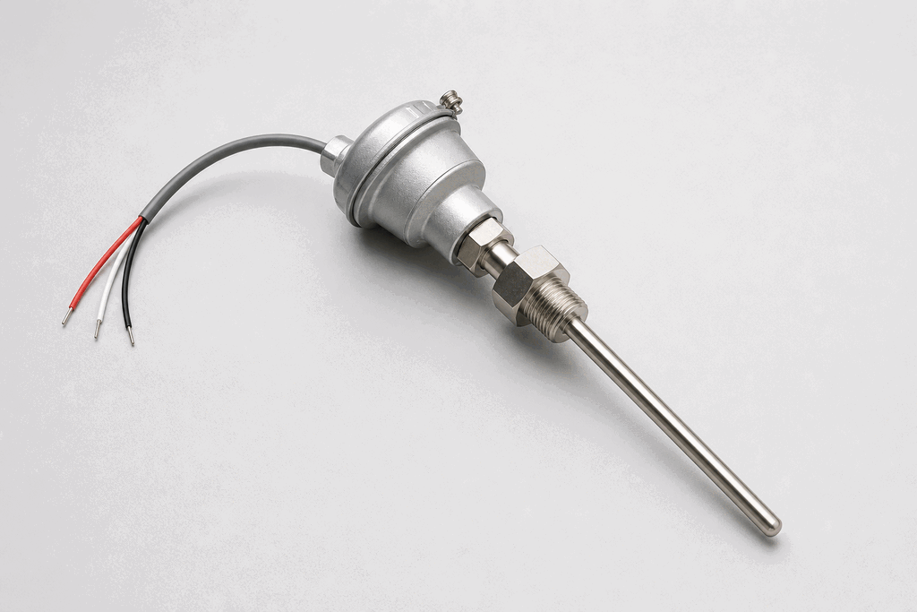
Representative real-world RTD / PT100 Temperature Sensor hardware on an industrial workbench
Representative field appearance · form factors vary by manufacturer

Hardware recognition

Know what to look for

Use the silhouette, active face, and connection style to identify the device before checking its part number and datasheet.

Body and mounting
A stainless probe often looks similar to a thermocouple assembly.
Active face
The platinum element is protected inside the probe tip.
Cable and terminals
Two-, three-, or four-wire terminals distinguish the lead-compensation method.
Field rule: identify by appearance, then verify the exact wiring, range, approvals, and output type from the device label and datasheet.

02 / Understand the principle

Watch cause become a PLC signal

Follow the physical event through the sensing element and into the exact controller value.

Signal story / live loop

RTD / PT100 Temperature Sensor: cause to controller

Paused

Now showingPhysical event

Probe temperature rises → Resistance increases → %IW68 = 180 °C

03 / Test and commission it

Commission it on the bench

Move the process, adjust the setpoint, invert the logic and inject faults. Watch the PLC value respond immediately.

Commissioning bench

RTD / PT100 Temperature Sensor

24 VDC%IW68
9.60 mA
108 °C
180 °C

PLC channel

%IW68

RAW 9677

Engineering value

108 °C

RTD input

Output logic
Inject a field fault

Channel healthy

Signal is inside the expected operating range

Terminals
Excitation +Sense +Return −

Commissioning note: A 3-wire input compensates lead resistance only when lead lengths and gauges match.

Field guide

An RTD (Resistance Temperature Detector) measures temperature by exploiting the predictable increase in electrical resistance of a metal element as temperature rises. PT100 — the most common industrial type — uses a platinum element with a resistance of exactly 100 Ω at 0 °C. At 100 °C the resistance is approximately 138.5 Ω; the relationship is defined by the IEC 60751 standard (the α = 0.00385 Ω/Ω/°C coefficient curve).

**RTD vs Thermocouple — the core trade-off:** - **Accuracy:** PT100 offers ±0.15 °C (Class AA) to ±0.5 °C (Class B) accuracy. A Type K thermocouple is typically ±1.5 °C to ±2.5 °C. For processes where 1 °C matters, the RTD wins decisively. - **Range:** Thermocouples cover -200 °C to +1260 °C (Type K). PT100 covers -200 °C to +850 °C. For temperatures above 600 °C (furnaces, kilns, exhaust gas), a thermocouple is the only option. - **Linearity:** Platinum resistance vs temperature is nearly linear over the industrial range. Thermocouple output is nonlinear and requires a polynomial correction table in the module. - **Stability:** PT100 sensors drift less than 0.1 °C per year at moderate temperatures. High-temperature thermocouples can drift several degrees per year. - **Cost:** RTD sensors and their input modules cost more than thermocouple equivalents. For high-density temperature monitoring (10+ points), the cost differential becomes significant.

**2-wire, 3-wire, and 4-wire configurations** exist because the lead resistance of the cable between the RTD and the PLC module adds to the measured resistance, introducing a temperature error:

- **2-wire:** the cable resistance is included in the measurement. Accurate only for very short cable runs (<1 m) or when cable resistance is calibrated out. Avoid in industrial settings. - **3-wire:** the most common industrial configuration. A third conductor allows the module to measure and subtract the lead resistance. Eliminates most lead-resistance error assuming the three conductors have equal resistance (same gauge, same length, same temperature). - **4-wire (Kelvin):** true four-wire measurement. Two wires carry the excitation current; two separate wires measure the voltage drop across the element only. Lead resistance has zero effect. Used in precision laboratory and pharmaceutical applications. Requires a 4-wire RTD input channel.

**PLC wiring:** RTD input modules (e.g. Siemens SM331 RTD, Allen-Bradley 1756-IR6I) supply a precise excitation current to the RTD and measure the resulting voltage. The module applies the IEC 60751 linearisation and outputs a scaled integer — typically 0 to 27648 representing 0.0 °C to a configurable upper range. Shielded cable, grounded at the panel end only, is mandatory for accurate low-resistance measurement.
Use this when…

  • Process temperature measurement requiring ±0.5 °C or better accuracy
  • Long cable runs where thermocouple extension wire cost or signal noise is a concern
  • Food, pharmaceutical, or water treatment where stability and repeatability over years matter

Where you will see it

Pharmaceutical batch reactor

PT100 sensors in a 4-wire configuration measure batch temperature to ±0.3 °C for GMP process validation — the linearity of platinum means calibration drift over a 5-year service life is negligible.

Water treatment

PT100 sensors monitor inlet/outlet temperatures on heat exchangers; the small temperature differences (2–5 °C) require the accuracy class that thermocouples cannot reliably achieve.

PLC wiring reference

Trace the complete electrical path instead of treating the PLC tag as magic. Confirm the device datasheet before wiring real hardware.

  1. 1Excitation +
  2. 2Sense +
  3. 3Return −

Commissioning checkpoint

A 3-wire input compensates lead resistance only when lead lengths and gauges match.

PLC address
%IW68
Expected signal
RTD input

Field questions

Frequently asked questions

What signal does a RTD / PT100 Temperature Sensor send to a PLC?

RTD input is read at %IW68. The exact electrical connection is Excitation +, Sense +, Return −.

How do you commission a RTD / PT100 Temperature Sensor?

A 3-wire input compensates lead resistance only when lead lengths and gauges match.

Next skill

Connect it to PLC logic

Unlock PLC integration challenges

See plans

Free first success

Use the rtd / pt100 temperature sensor signal in PLC logic

Apply the wiring and commissioning model in a scored browser exercise, then save your progress and continue through the recommended path.

No installNo credit cardImmediate pass/fail feedback

Technical reference and worked-example guide

RTD and Pt100 sensor guide: implementation, evidence and troubleshooting

Direct answer

RTD and Pt100 sensor guide becomes useful when it connects rtd type, element curve, wire count, range, transmitter, supply, input mode, units, accuracy and calibration points with temperature through sensor resistance, lead wires, transmitter or rtd module, raw value and scaled plc tag, then proves known low, midpoint and high temperatures producing coherent resistance, loop and engineering values under normal, boundary, fault and recovery conditions. The objective is a repeatable engineering or learning result, not merely activity inside a page or tool.

This guide is written for instrumentation and PLC learners comparing Pt100 wiring, lead compensation, transmitter conversion, analog input scaling and fault evidence. The intended result is specific: the learner can trace temperature through resistance, wiring or transmitter, input counts and engineering units and can prove low, midpoint and high values.

Instrumentation technician checking an RTD, transmitter, isolated barrier and PLC analog input at several calibration points
Commission the complete temperature signal chain at known low, midpoint and high conditions.

System map / 02

Six concepts that control the result

Treat these as connected checkpoints. Each checkpoint has an expected state, an observable state and a boundary to the next part of the system. That structure prevents a software indication from being mistaken for physical proof.

NODE 01observable

Define the operating contract

RTD type, element curve, wire count, range, transmitter, supply, input mode, units, accuracy and calibration points. For RTD temperature measurement and PLC scaling, record the initial condition, actor, requested change, observable result and stopping condition before selecting a tool or implementation.

NODE 02observable

Map the evidence path

temperature through sensor resistance, lead wires, transmitter or RTD module, raw value and scaled PLC tag. Separate request, internal state, output or service, physical or user-visible result and independent feedback so each boundary can be inspected.

NODE 03observable

Prove normal operation

known low, midpoint and high temperatures producing coherent resistance, loop and engineering values. Run more than one cycle from a known state and retain the values, timings or artifacts that demonstrate repeatability.

NODE 04observable

Exercise a boundary case

lead resistance, open circuit, short circuit, wrong wiring mode, transmitter range, noise and out-of-range. Choose minimum, maximum, simultaneous, delayed or restart conditions that reveal assumptions hidden by the happy path.

NODE 05observable

Diagnose a controlled fault

a sensor, lead, terminal, transmitter, input configuration, scaling or units defect. Preserve the first symptom, divide the system at a measurable boundary and change one condition only after predicting the result.

NODE 06observable

Transfer and hand over

the loop checked with traceable equipment and exact device and module documentation. Restore normal state, remove temporary changes, repeat affected checks and document which claims remain limited to the learning environment.

Procedure / 03

A six-step practice and commissioning workflow

Run the steps in order the first time. Later, the same structure becomes a diagnostic loop: define the expected condition, observe the boundary, interpret the difference and choose one proving action.

  1. 01

    Write the acceptance case

    Convert rtd type, element curve, wire count, range, transmitter, supply, input mode, units, accuracy and calibration points into initial conditions, one stimulus and observable pass criteria.

    Evidence: Another person can repeat the case without guessing the intended result.

    Avoid: Using page completion or an animation as the acceptance criterion.

  2. 02

    Build the map

    Document temperature through sensor resistance, lead wires, transmitter or rtd module, raw value and scaled plc tag and name who owns each state or decision.

    Evidence: Every request and result has a source, destination and useful inspection point.

    Avoid: Using the same value as command, status and independent feedback.

  3. 03

    Run the baseline

    Apply known low, midpoint and high temperatures producing coherent resistance, loop and engineering values from a clean start and record the expected evidence.

    Evidence: Repeated runs produce the same bounded result.

    Avoid: Changing several parameters before a baseline exists.

  4. 04

    Challenge assumptions

    Test lead resistance, open circuit, short circuit, wrong wiring mode, transmitter range, noise and out-of-range without changing the acceptance contract.

    Evidence: Limits, timing and restart behavior reach defined states.

    Avoid: Testing only one ideal sequence.

  5. 05

    Isolate one failure

    Introduce or analyse a sensor, lead, terminal, transmitter, input configuration, scaling or units defect and locate the first disagreement.

    Evidence: The proving action distinguishes the leading hypotheses.

    Avoid: Resetting, forcing or replacing before evidence is retained.

  6. 06

    Close the evidence loop

    Complete the loop checked with traceable equipment and exact device and module documentation and repeat the affected regression cases.

    Evidence: Reference use is complete when inputs, assumptions, units or initial conditions are recorded and the result is independently checked at a useful boundary.

    Avoid: Treating an acknowledged message or one successful rerun as handover.

Diagnostic matrix / 04

Symptoms, proving points and next actions

The table is a reasoning aid, not a parts-replacement chart. Preserve the initial symptom, inspect the named boundary and use the interpretation to choose the next controlled test. Site safety procedures and equipment manuals remain authoritative.

Diagnostic symptoms, inspection points, interpretations and next actions for RTD and Pt100 sensor guide: implementation, evidence and troubleshooting
Observed symptomInspectInterpretationNext proving action
The expected result is unclearRequirement, initial state, actor, stimulus, units and pass conditionThe technician, programmer and reviewer may be solving different versions of the task.Rewrite one observable acceptance case before continuing.
Internal state changes but the outcome does notRequest, final owner, output or service boundary and independent feedbackA software or interface indication proves intent at one layer, not the complete outcome.Trace the first boundary after the changing state.
Normal case passes but an edge case failsLimits, timing, simultaneous events, reset and restart assumptionsThe implementation contains a hidden assumption exposed by the changed condition.Add the failed boundary as a permanent regression case.
The failure disappears after resetOriginal symptom, histories, diagnostics, timestamps and active causeReset changed evidence or state without proving the initiating cause.Reproduce under a controlled condition and preserve pre/post-event data.
Simulator and target disagreeModel boundary, software version, task timing, I/O behavior, data types and configurationA learning model and the intended target do not share one of the recorded assumptions.Reduce the case and verify against current target documentation.
The result cannot be explainedPrediction, observation, proving action, alternative hypotheses and limitationsActivity occurred but the evidence is not yet transferable or reviewable.Have the learner defend the signal path and repeat a changed case.

Product evidence / 05

What the browser practice can actually demonstrate

The page connects definitions and worked examples to runnable tools, explicit assumptions and repeatable checks so a formula or pattern can be challenged.

Where simulation stops

The lesson does not establish calibration authority, hazardous-area suitability, wiring practice or measurement uncertainty for an installed loop.

Commissioning notebook / 06

Six cases that turn the concepts into evidence

Use these as written briefs rather than click-through instructions. For every case, state the expected condition before acting, retain the first useful observation and explain why the final result proves the requirement. A different program or component choice can still be correct when it produces the same bounded behavior and evidence.

Case 01

predict → observe → prove

Prove define the operating contract

Engineering context. RTD type, element curve, wire count, range, transmitter, supply, input mode, units, accuracy and calibration points. For RTD temperature measurement and PLC scaling, record the initial condition, actor, requested change, observable result and stopping condition before selecting a tool or implementation. Begin with a written normal condition and identify which request, state, physical result or communication value will provide independent confirmation. Do not begin by changing the configuration; the initial state is part of the evidence and should remain reproducible.

Controlled setup. Use the “Write the acceptance case” stage of the workflow: convert rtd type, element curve, wire count, range, transmitter, supply, input mode, units, accuracy and calibration points into initial conditions, one stimulus and observable pass criteria. The acceptance record should show this result: another person can repeat the case without guessing the intended result. Record initial conditions, the exact stimulus and the observation point so another learner can repeat the case without relying on your memory.

Fault challenge. Introduce or analyse “The expected result is unclear” as one bounded deviation. Inspect requirement, initial state, actor, stimulus, units and pass condition The working interpretation is that the technician, programmer and reviewer may be solving different versions of the task. The next proving action is to rewrite one observable acceptance case before continuing. Change only one condition before observing the result, and preserve timestamps or measurements where timing matters.

Review and recovery. The most common trap here is using page completion or an animation as the acceptance criterion. After restoring the cause, repeat the normal case and at least one stop, timeout, disconnect or restart boundary relevant to this topic. Remove temporary forces and bypasses, return the model to a known state and retain the evidence that both operation and recovery are deliberate.

Explain it aloud: What should I learn first about RTD temperature measurement and PLC scaling? A defensible short answer is: Start with the operating contract and evidence path: rtd type, element curve, wire count, range, transmitter, supply, input mode, units, accuracy and calibration points, followed by temperature through sensor resistance, lead wires, transmitter or rtd module, raw value and scaled plc tag. Add advanced features only after the baseline is predictable.

Case 02

predict → observe → prove

Prove map the evidence path

Engineering context. temperature through sensor resistance, lead wires, transmitter or RTD module, raw value and scaled PLC tag. Separate request, internal state, output or service, physical or user-visible result and independent feedback so each boundary can be inspected. Begin with a written normal condition and identify which request, state, physical result or communication value will provide independent confirmation. Do not begin by changing the configuration; the initial state is part of the evidence and should remain reproducible.

Controlled setup. Use the “Build the map” stage of the workflow: document temperature through sensor resistance, lead wires, transmitter or rtd module, raw value and scaled plc tag and name who owns each state or decision. The acceptance record should show this result: every request and result has a source, destination and useful inspection point. Record initial conditions, the exact stimulus and the observation point so another learner can repeat the case without relying on your memory.

Fault challenge. Introduce or analyse “Internal state changes but the outcome does not” as one bounded deviation. Inspect request, final owner, output or service boundary and independent feedback The working interpretation is that a software or interface indication proves intent at one layer, not the complete outcome. The next proving action is to trace the first boundary after the changing state. Change only one condition before observing the result, and preserve timestamps or measurements where timing matters.

Review and recovery. The most common trap here is using the same value as command, status and independent feedback. After restoring the cause, repeat the normal case and at least one stop, timeout, disconnect or restart boundary relevant to this topic. Remove temporary forces and bypasses, return the model to a known state and retain the evidence that both operation and recovery are deliberate.

Explain it aloud: How do I practise RTD temperature measurement and PLC scaling effectively? A defensible short answer is: Use short cases with known initial conditions, a written prediction, one action and an observable result. Then alter a boundary or fault and explain why the evidence changed.

Case 03

predict → observe → prove

Prove prove normal operation

Engineering context. known low, midpoint and high temperatures producing coherent resistance, loop and engineering values. Run more than one cycle from a known state and retain the values, timings or artifacts that demonstrate repeatability. Begin with a written normal condition and identify which request, state, physical result or communication value will provide independent confirmation. Do not begin by changing the configuration; the initial state is part of the evidence and should remain reproducible.

Controlled setup. Use the “Run the baseline” stage of the workflow: apply known low, midpoint and high temperatures producing coherent resistance, loop and engineering values from a clean start and record the expected evidence. The acceptance record should show this result: repeated runs produce the same bounded result. Record initial conditions, the exact stimulus and the observation point so another learner can repeat the case without relying on your memory.

Fault challenge. Introduce or analyse “Normal case passes but an edge case fails” as one bounded deviation. Inspect limits, timing, simultaneous events, reset and restart assumptions The working interpretation is that the implementation contains a hidden assumption exposed by the changed condition. The next proving action is to add the failed boundary as a permanent regression case. Change only one condition before observing the result, and preserve timestamps or measurements where timing matters.

Review and recovery. The most common trap here is changing several parameters before a baseline exists. After restoring the cause, repeat the normal case and at least one stop, timeout, disconnect or restart boundary relevant to this topic. Remove temporary forces and bypasses, return the model to a known state and retain the evidence that both operation and recovery are deliberate.

Explain it aloud: What counts as proof of competence? A defensible short answer is: A repeatable artifact or system result plus an explanation of the signal path is stronger than time spent, screenshots or a copied answer. Physical competence requires separate supervised evidence.

Case 04

predict → observe → prove

Prove exercise a boundary case

Engineering context. lead resistance, open circuit, short circuit, wrong wiring mode, transmitter range, noise and out-of-range. Choose minimum, maximum, simultaneous, delayed or restart conditions that reveal assumptions hidden by the happy path. Begin with a written normal condition and identify which request, state, physical result or communication value will provide independent confirmation. Do not begin by changing the configuration; the initial state is part of the evidence and should remain reproducible.

Controlled setup. Use the “Challenge assumptions” stage of the workflow: test lead resistance, open circuit, short circuit, wrong wiring mode, transmitter range, noise and out-of-range without changing the acceptance contract. The acceptance record should show this result: limits, timing and restart behavior reach defined states. Record initial conditions, the exact stimulus and the observation point so another learner can repeat the case without relying on your memory.

Fault challenge. Introduce or analyse “The failure disappears after reset” as one bounded deviation. Inspect original symptom, histories, diagnostics, timestamps and active cause The working interpretation is that reset changed evidence or state without proving the initiating cause. The next proving action is to reproduce under a controlled condition and preserve pre/post-event data. Change only one condition before observing the result, and preserve timestamps or measurements where timing matters.

Review and recovery. The most common trap here is testing only one ideal sequence. After restoring the cause, repeat the normal case and at least one stop, timeout, disconnect or restart boundary relevant to this topic. Remove temporary forces and bypasses, return the model to a known state and retain the evidence that both operation and recovery are deliberate.

Explain it aloud: Why test faults and restart behavior? A defensible short answer is: Because a sensor, lead, terminal, transmitter, input configuration, scaling or units defect or lead resistance, open circuit, short circuit, wrong wiring mode, transmitter range, noise and out-of-range can expose assumptions that never appear during ideal startup and steady operation.

Case 05

predict → observe → prove

Prove diagnose a controlled fault

Engineering context. a sensor, lead, terminal, transmitter, input configuration, scaling or units defect. Preserve the first symptom, divide the system at a measurable boundary and change one condition only after predicting the result. Begin with a written normal condition and identify which request, state, physical result or communication value will provide independent confirmation. Do not begin by changing the configuration; the initial state is part of the evidence and should remain reproducible.

Controlled setup. Use the “Isolate one failure” stage of the workflow: introduce or analyse a sensor, lead, terminal, transmitter, input configuration, scaling or units defect and locate the first disagreement. The acceptance record should show this result: the proving action distinguishes the leading hypotheses. Record initial conditions, the exact stimulus and the observation point so another learner can repeat the case without relying on your memory.

Fault challenge. Introduce or analyse “Simulator and target disagree” as one bounded deviation. Inspect model boundary, software version, task timing, I/O behavior, data types and configuration The working interpretation is that a learning model and the intended target do not share one of the recorded assumptions. The next proving action is to reduce the case and verify against current target documentation. Change only one condition before observing the result, and preserve timestamps or measurements where timing matters.

Review and recovery. The most common trap here is resetting, forcing or replacing before evidence is retained. After restoring the cause, repeat the normal case and at least one stop, timeout, disconnect or restart boundary relevant to this topic. Remove temporary forces and bypasses, return the model to a known state and retain the evidence that both operation and recovery are deliberate.

Explain it aloud: Can browser practice replace official software or hardware? A defensible short answer is: No. It can build concepts and diagnostic reasoning. Exact firmware, I/O electrical behavior, networking, safety and commissioning require current official tools, documentation and target equipment.

Case 06

predict → observe → prove

Prove transfer and hand over

Engineering context. the loop checked with traceable equipment and exact device and module documentation. Restore normal state, remove temporary changes, repeat affected checks and document which claims remain limited to the learning environment. Begin with a written normal condition and identify which request, state, physical result or communication value will provide independent confirmation. Do not begin by changing the configuration; the initial state is part of the evidence and should remain reproducible.

Controlled setup. Use the “Close the evidence loop” stage of the workflow: complete the loop checked with traceable equipment and exact device and module documentation and repeat the affected regression cases. The acceptance record should show this result: reference use is complete when inputs, assumptions, units or initial conditions are recorded and the result is independently checked at a useful boundary. Record initial conditions, the exact stimulus and the observation point so another learner can repeat the case without relying on your memory.

Fault challenge. Introduce or analyse “The result cannot be explained” as one bounded deviation. Inspect prediction, observation, proving action, alternative hypotheses and limitations The working interpretation is that activity occurred but the evidence is not yet transferable or reviewable. The next proving action is to have the learner defend the signal path and repeat a changed case. Change only one condition before observing the result, and preserve timestamps or measurements where timing matters.

Review and recovery. The most common trap here is treating an acknowledged message or one successful rerun as handover. After restoring the cause, repeat the normal case and at least one stop, timeout, disconnect or restart boundary relevant to this topic. Remove temporary forces and bypasses, return the model to a known state and retain the evidence that both operation and recovery are deliberate.

Explain it aloud: How should progress be documented? A defensible short answer is: Keep the requirement, initial state, program or configuration, observed values, fault hypothesis, proving action, recovery result and a concise limitations statement.

Answer surface / 07

Questions people ask about RTD and Pt100 sensor guide

These concise answers define the operating, training and product boundaries most often missed in broad summaries. The full workflow and diagnostic table above provide the evidence behind them.

What should I learn first about RTD temperature measurement and PLC scaling?

Start with the operating contract and evidence path: rtd type, element curve, wire count, range, transmitter, supply, input mode, units, accuracy and calibration points, followed by temperature through sensor resistance, lead wires, transmitter or rtd module, raw value and scaled plc tag. Add advanced features only after the baseline is predictable.

How do I practise RTD temperature measurement and PLC scaling effectively?

Use short cases with known initial conditions, a written prediction, one action and an observable result. Then alter a boundary or fault and explain why the evidence changed.

What counts as proof of competence?

A repeatable artifact or system result plus an explanation of the signal path is stronger than time spent, screenshots or a copied answer. Physical competence requires separate supervised evidence.

Why test faults and restart behavior?

Because a sensor, lead, terminal, transmitter, input configuration, scaling or units defect or lead resistance, open circuit, short circuit, wrong wiring mode, transmitter range, noise and out-of-range can expose assumptions that never appear during ideal startup and steady operation.

Can browser practice replace official software or hardware?

No. It can build concepts and diagnostic reasoning. Exact firmware, I/O electrical behavior, networking, safety and commissioning require current official tools, documentation and target equipment.

How should progress be documented?

Keep the requirement, initial state, program or configuration, observed values, fault hypothesis, proving action, recovery result and a concise limitations statement.

What should I do when the answer differs from a guide?

Check assumptions, version, units and initial state first. Reduce the case, compare one boundary at a time and prefer current primary documentation for target-specific behavior.

When is a RTD temperature measurement and PLC scaling exercise finished?

Reference use is complete when inputs, assumptions, units or initial conditions are recorded and the result is independently checked at a useful boundary.

Real pt100 rtd sensor footage

See this exact skill in the working simulator.

Watch the real browser product respond to the task on this page, then try the same practical workflow yourself. No slides, concept mockups, install, or credit card.

Try this in the browser
PT100 RTD Sensor — Resistance, Wiring and PLC Scaling