Pro
35 min

Sorting Machine PLC Program & Ladder Diagram

This page covers the full sorting machine PLC program and ladder diagram — metal-versus-plastic part sorting using an inductive sensor, a pneumatic reject gate, a CTU production counter, and a safety interlock that keeps the gate from firing while a part still breaks the entry beam. It is grounded in a live scenario you can run directly in your browser: write the ladder, watch parts travel and sort, and get instant pass/fail feedback — no PLC hardware, no software install. It is runnable and auto-graded free.

sensorscounterssorting
Sorting Machine scenario preview

Ready to build this?

Sign up free — no credit card required. This scenario requires the Pro plan.

Sign up to play this scenario →

Already have an account? Log in

Briefing

Mixed parts travel along a sorting belt. An entry photo-eye announces each arriving part. An inductive METAL_SENSOR further down the line fires only for metal parts — plastic parts pass it without a signal. Metal parts must be diverted onto a reject lane by firing REJECT_GATE while the part is passing the diverter arm; plastic parts continue straight. A counter watches the reject lane's limit sensor and lights METAL_COUNT_LAMP once five metal parts have been rejected.

Objectives

  • START energises BELT; STOP de-energises it
  • Fire REJECT_GATE so that metal parts are pushed onto the reject lane
  • Leave REJECT_GATE off for plastic parts
  • Light METAL_COUNT_LAMP once 5 metal parts have cleared the reject-lane limit sensor
  • Never energise REJECT_GATE while PART_PE is still broken — the arm would collide with the part

Hints

  • Use SET/RESET on BELT driven by START (set) and STOP (reset)
  • SET REJECT_GATE on METAL_SENSOR and RESET it on REJECT_LIMIT — the belt spacing guarantees PART_PE has already cleared before METAL_SENSOR fires
  • Count REJECT_LIMIT rising edges with a CTU (PV := 5) and drive METAL_COUNT_LAMP from its Q output
  • Plastic parts never trip METAL_SENSOR, so the same gate logic leaves them untouched — no separate plastic branch is needed

I/O Table

Inputs

START

Start push-button (momentary)

BOOL · %I0.0

STOP

Stop push-button (momentary)

BOOL · %I0.1

PART_PE

Entry photo-eye (beam broken by any part)

BOOL · %I0.2

METAL_SENSOR

Inductive sensor (true only for metal parts)

BOOL · %I0.3

REJECT_LIMIT

Reject-lane limit sensor

BOOL · %I0.4

Outputs

BELT

Sorting belt motor contactor

BOOL · %Q0.0

REJECT_GATE

Pneumatic reject-gate solenoid (diverts metal)

BOOL · %Q0.1

METAL_COUNT_LAMP

Metal count ≥ 5 indicator

BOOL · %Q0.2

Your program will be tested against:

All test cases run automatically when you submit. Assertions are hidden until you pass.

  1. #1Metal part fires the reject gate and is diverted

    Inject a metal part: gate energises across the transit window, part reaches the reject lane

  2. #2Start energises the belt, stop drops it

    START -> BELT on; STOP -> off

  3. #3Plastic part passes without firing the reject gate

    Inject a plastic part: reject gate remains off throughout the run

  4. #4Five metal parts light METAL_COUNT_LAMP

    Five metal parts injected spaced apart; METAL_COUNT_LAMP energises after the fifth is rejected

  5. #5Reject gate never fires while a part still breaks the entry beam

    Inject a metal part; assert the gate was never energised while PART_PE was active

How a sorting machine PLC program works

A sorting machine moves mixed parts along a belt and diverts one category onto a reject lane while letting the rest pass straight through. In this scenario the discriminator is material: metal parts must be rejected, plastic parts pass. Object sorting using a PLC comes down to four jobs — run the belt, detect the part type, fire a diverter at the right moment, and count what was sorted.

The belt is the foundation. START energises BELT and STOP de-energises it — a standard motor start/stop you can build with a SET/RESET pair on BELT driven by START (set) and STOP (reset).

Detection uses two sensors in sequence. PART_PE (%I0.2) is an entry photo-eye whose beam is broken by any arriving part — metal or plastic. Further down the line, METAL_SENSOR (%I0.3) is an inductive sensor that fires only for metal: plastic parts pass it without ever producing a signal. That is the whole material discrimination — no separate plastic branch is needed, because plastic simply never trips the inductive sensor.

The diverter is REJECT_GATE (%Q0.1), a pneumatic solenoid that pushes a part onto the reject lane. REJECT_LIMIT (%I0.4) is the limit sensor at the reject lane that confirms a part has been pushed across. Finally, METAL_COUNT_LAMP (%Q0.2) lights once five metal parts have been rejected. Five inputs, three outputs — all pre-wired for you.

Metal-vs-plastic sorting with an inductive sensor and reject gate

The sort logic is one latch. SET REJECT_GATE when METAL_SENSOR detects metal; RESET REJECT_GATE when REJECT_LIMIT confirms the part has reached the reject lane. While the gate is set, the pneumatic arm is extended and pushes the metal part off the main belt; once REJECT_LIMIT trips, the part is clear and the gate retracts ready for the next one.

This is the elegant part of inductive sensor PLC sorting: the same single rung handles both materials. A metal part trips METAL_SENSOR, so the gate fires and diverts it. A plastic part never trips METAL_SENSOR, so the gate stays off and the part rides straight through to the end of the belt. You do not write a 'plastic' rung at all — the absence of an inductive signal is the plastic case.

Two test cases pin this down. The discriminating 'metal-part-diverts' case injects a metal part and checks the gate is still off before the part reaches METAL_SENSOR (~2 s in), energised after METAL_SENSOR fires (~4 s), and dropped again after REJECT_LIMIT (~6 s) — and that the physics counted exactly one rejected metal part. The 'plastic-part-passes' case injects a plastic part, lets it traverse the entire belt, and asserts REJECT_GATE never energised and the metal-rejected count stayed at zero. Get the SET sensor wrong — fire on PART_PE instead of METAL_SENSOR — and the plastic test fails because the gate would divert everything.

Counting rejects with a CTU — lighting the lamp after five metal parts

Once the gate is sorting correctly, the metal sorting PLC program needs a production count: light METAL_COUNT_LAMP after five metal parts have been rejected. This is a textbook CTU (count-up) application.

Add a CTU with its preset (PV) set to 5. Drive the count-up input from REJECT_LIMIT — but through a rising-edge detector. REJECT_LIMIT is a level signal: it stays true for as long as a part is physically over the limit sensor. Feed that level straight into the CTU and the counter would increment on every scan the sensor is blocked, adding dozens of spurious counts per part. An R_TRIG (or equivalent one-shot) converts the level to a single pulse, giving you exactly one count per rejected part.

Wire the CTU's done output (CTU.Q in IEC, CTU.DN in Allen-Bradley) to METAL_COUNT_LAMP. When the accumulator reaches 5 the done bit goes true and the lamp lights.

The 'counter' test injects five metal parts spaced seven seconds apart — wide enough that each part clears the entry beam before the next reaches the inductive sensor. It asserts METAL_COUNT_LAMP is still off after the fourth part has been rejected and on after the fifth, and it checks the physics engine's metalRejectedCount is exactly 5. Because plastic parts never reach the reject lane, they never trip REJECT_LIMIT and never inflate the count — the counter inherently tallies only metal.

The safety interlock — never fire the gate while the entry beam is broken

Every diverter on a sorting line has the same mechanical hazard: if the reject gate extends while a part is still partly over the arm's pivot, the arm slams into the part and jams the machine. The safety rule, stated as an objective, is that REJECT_GATE must never energise while PART_PE — the entry photo-eye — is still broken.

The scenario's belt spacing makes the safe design natural rather than fiddly. By the time a part travels far enough down the belt to reach METAL_SENSOR, it has already cleared the entry photo-eye, so PART_PE is no longer broken. That is exactly why the sort latch is built to SET REJECT_GATE on METAL_SENSOR and not on PART_PE: firing on the inductive sensor guarantees the part is already past the entry beam. If instead you fired the gate the instant PART_PE detected a part, the arm could collide with the part while it is still entering — the violation the interlock exists to prevent.

The 'safety-invariant' test injects a metal part, lets it run the full length of the belt past REJECT_LIMIT, and then asserts the physics flag rejectWhileEntryViolation is false — i.e. at no point during the run was the gate energised while PART_PE was still broken. A solution that sorts correctly on count and material but fires the gate too early will pass the divert and counter tests yet fail this one.

The whole sorting machine PLC ladder diagram is runnable and auto-graded on this page. Write it, press Run, and watch metal parts divert onto the reject lane while plastic parts pass — with five automated test cases grading the belt, the metal divert, the plastic pass-through, the five-count lamp, and the entry-beam safety interlock. No physical PLC, conveyor or sensors required.

Frequently asked questions

How does a PLC sorting machine separate metal from plastic?

It uses an inductive proximity sensor, which produces a signal only when a metal part passes in front of it — plastic parts pass without any signal. The PLC program latches a reject-gate solenoid on when the inductive sensor fires and resets it when a reject-lane limit sensor confirms the part has been pushed across. Metal parts trip the inductive sensor and get diverted; plastic parts never trip it, so the gate stays off and they pass straight through. No separate plastic-detection logic is needed.

What ladder logic does a sorting machine PLC program use?

A sorting machine PLC ladder diagram uses a SET/RESET pair on the belt motor (SET on START, RESET on STOP), a SET/RESET pair on the reject-gate solenoid (SET when the inductive metal sensor fires, RESET when the reject-lane limit sensor confirms the divert), and a CTU count-up counter fed by a rising-edge detector on the limit sensor to tally rejected parts. The CTU done bit drives the count lamp once the preset (for example 5) is reached.

How do you count sorted parts in a PLC program?

Add a CTU (count-up) counter with its preset set to the target — for example 5. Drive the count-up input from the reject-lane limit sensor through a rising-edge detector (R_TRIG) so the counter increments exactly once per part rather than once per scan while the sensor is blocked. Wire the CTU done output (CTU.Q in IEC, CTU.DN in Allen-Bradley) to the indicator lamp; it lights when the accumulator reaches the preset. Because only diverted metal parts reach the limit sensor, the counter inherently tallies metal only.

What is the safety interlock in a sorting machine PLC program?

The reject gate must never extend while a part is still breaking the entry photo-eye, or the pneumatic arm collides with the part and jams the machine. The safe design sets the gate on the inductive metal sensor rather than the entry photo-eye: by the time a part reaches the metal sensor further down the belt, it has already cleared the entry beam. The scenario verifies this with a test that injects a metal part and asserts the gate was never energised while the entry beam was still broken.

Can I simulate a sorting machine PLC program without hardware?

Yes. The Sorting Machine scenario on this page runs directly in your browser — write the ladder logic, press Run, and watch metal parts divert onto a reject lane while plastic parts pass straight through. The physics engine moves parts at a realistic belt speed and fires the photo-eye, inductive sensor and limit sensor at the correct positions, and the auto-grader checks the belt start/stop, the metal divert, the plastic pass-through, the five-part count lamp, and the entry-beam safety interlock. No physical PLC, conveyor or sensors required.

Ready to build this?

Sign up free — no credit card required. This scenario requires the Pro plan.

Sign up to play this scenario →

Already have an account? Log in

Runnable simulator field guide

Sorting machine PLC scenario: implementation, evidence and troubleshooting

Direct answer

Sorting machine PLC scenario becomes useful when it connects product classes, sensor positions, conveyor speed, travel distance, tracking identity, actuator delay, reject destination, confirmation, timeout, counters and reset policy with item arrival through detection, classification, queue or shift register, calculated actuation point, diverter command, destination feedback and production counts, then proves mixed items are classified, tracked and routed once with no double count or stale product identity under normal, boundary, fault and recovery conditions. The objective is a repeatable engineering or learning result, not merely activity inside a page or tool.

This guide is written for pLC learners building photoeye detection, item classification, conveyor tracking, actuator timing, reject confirmation, counts, jams and safe recovery. The intended result is specific: the learner can follow one item from detection through classification and tracked position to the correct diverter action and independently confirmed destination.

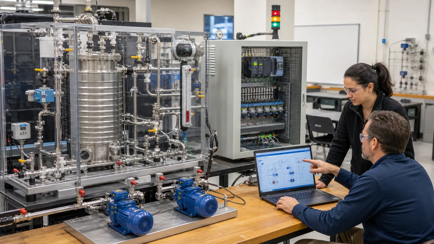
an instructor and technician validating chiller and duty-standby pump control on a stainless process training rig with visible instruments and feedback while studying conveyor sorting sequence, tracking and reject evidence
The scene keeps conveyor sorting sequence, tracking and reject evidence connected to a declared operating condition, observable evidence, safe boundaries and a result another person can reproduce.

System map / 02

Six concepts that control the result

Treat these as connected checkpoints. Each checkpoint has an expected state, an observable state and a boundary to the next part of the system. That structure prevents a software indication from being mistaken for physical proof.

NODE 01observable

Define the operating contract

product classes, sensor positions, conveyor speed, travel distance, tracking identity, actuator delay, reject destination, confirmation, timeout, counters and reset policy. For conveyor sorting sequence, tracking and reject evidence, record the initial condition, actor, requested change, observable result and stopping condition before selecting a tool or implementation.

NODE 02observable

Map the evidence path

item arrival through detection, classification, queue or shift register, calculated actuation point, diverter command, destination feedback and production counts. Separate request, internal state, output or service, physical or user-visible result and independent feedback so each boundary can be inspected.

NODE 03observable

Prove normal operation

mixed items are classified, tracked and routed once with no double count or stale product identity. Run more than one cycle from a known state and retain the values, timings or artifacts that demonstrate repeatability.

NODE 04observable

Exercise a boundary case

back-to-back products, sensor chatter, speed change, unknown class, jam, missed feedback, full reject bin, stop and restart. Choose minimum, maximum, simultaneous, delayed or restart conditions that reveal assumptions hidden by the happy path.

NODE 05observable

Diagnose a controlled fault

a detection, classification, identity, position, timing, actuator, confirmation, count, jam or recovery mismatch. Preserve the first symptom, divide the system at a measurable boundary and change one condition only after predicting the result.

NODE 06observable

Transfer and hand over

timing and mechanics validated with target sensors, conveyor, actuator, guarding and measured product trials. Restore normal state, remove temporary changes, repeat affected checks and document which claims remain limited to the learning environment.

Procedure / 03

A six-step practice and commissioning workflow

Run the steps in order the first time. Later, the same structure becomes a diagnostic loop: define the expected condition, observe the boundary, interpret the difference and choose one proving action.

  1. 01

    Write the acceptance case

    Convert product classes, sensor positions, conveyor speed, travel distance, tracking identity, actuator delay, reject destination, confirmation, timeout, counters and reset policy into initial conditions, one stimulus and observable pass criteria.

    Evidence: Another person can repeat the case without guessing the intended result.

    Avoid: Using page completion or an animation as the acceptance criterion.

  2. 02

    Build the map

    Document item arrival through detection, classification, queue or shift register, calculated actuation point, diverter command, destination feedback and production counts and name who owns each state or decision.

    Evidence: Every request and result has a source, destination and useful inspection point.

    Avoid: Using the same value as command, status and independent feedback.

  3. 03

    Run the baseline

    Apply mixed items are classified, tracked and routed once with no double count or stale product identity from a clean start and record the expected evidence.

    Evidence: Repeated runs produce the same bounded result.

    Avoid: Changing several parameters before a baseline exists.

  4. 04

    Challenge assumptions

    Test back-to-back products, sensor chatter, speed change, unknown class, jam, missed feedback, full reject bin, stop and restart without changing the acceptance contract.

    Evidence: Limits, timing and restart behavior reach defined states.

    Avoid: Testing only one ideal sequence.

  5. 05

    Isolate one failure

    Introduce or analyse a detection, classification, identity, position, timing, actuator, confirmation, count, jam or recovery mismatch and locate the first disagreement.

    Evidence: The proving action distinguishes the leading hypotheses.

    Avoid: Resetting, forcing or replacing before evidence is retained.

  6. 06

    Close the evidence loop

    Complete timing and mechanics validated with target sensors, conveyor, actuator, guarding and measured product trials and repeat the affected regression cases.

    Evidence: A run is complete only when the requested behavior, stop behavior, fault response and recovery are observable from a fresh initial condition.

    Avoid: Treating an acknowledged message or one successful rerun as handover.

Diagnostic matrix / 04

Symptoms, proving points and next actions

The table is a reasoning aid, not a parts-replacement chart. Preserve the initial symptom, inspect the named boundary and use the interpretation to choose the next controlled test. Site safety procedures and equipment manuals remain authoritative.

Diagnostic symptoms, inspection points, interpretations and next actions for Sorting machine PLC scenario: implementation, evidence and troubleshooting
Observed symptomInspectInterpretationNext proving action
The expected result is unclearRequirement, initial state, actor, stimulus, units and pass conditionThe operator, programmer and reviewer may be solving different versions of the task.Rewrite one observable acceptance case before continuing.
Internal state changes but the outcome does notRequest, final owner, output or service boundary and independent feedbackA software or interface indication proves intent at one layer, not the complete outcome.Trace the first boundary after the changing state.
Normal case passes but an edge case failsLimits, timing, simultaneous events, reset and restart assumptionsThe implementation contains a hidden assumption exposed by the changed condition.Add the failed boundary as a permanent regression case.
The failure disappears after resetOriginal symptom, histories, diagnostics, timestamps and active causeReset changed evidence or state without proving the initiating cause.Reproduce under a controlled condition and preserve pre/post-event data.
Simulator and target disagreeModel boundary, software version, task timing, I/O behavior, data types and configurationA learning model and the intended target do not share one of the recorded assumptions.Reduce the case and verify against current target documentation.
The result cannot be explainedPrediction, observation, proving action, alternative hypotheses and limitationsActivity occurred but the evidence is not yet transferable or reviewable.Have the learner defend the signal path and repeat a changed case.

Product evidence / 05

What the browser practice can actually demonstrate

The browser runtime joins editable control state to visible I/O and machine or process behavior, allowing the same initial conditions and stimuli to be replayed.

Where simulation stops

The model cannot select real sensors or guards, predict product mechanics, validate stopping distance, calculate throughput or commission a physical sorting line.

Commissioning notebook / 06

Six cases that turn the concepts into evidence

Use these as written briefs rather than click-through instructions. For every case, state the expected condition before acting, retain the first useful observation and explain why the final result proves the requirement. A different program or component choice can still be correct when it produces the same bounded behavior and evidence.

Case 01

predict → observe → prove

Prove define the operating contract

Engineering context. product classes, sensor positions, conveyor speed, travel distance, tracking identity, actuator delay, reject destination, confirmation, timeout, counters and reset policy. For conveyor sorting sequence, tracking and reject evidence, record the initial condition, actor, requested change, observable result and stopping condition before selecting a tool or implementation. Begin with a written normal condition and identify which request, state, physical result or communication value will provide independent confirmation. Do not begin by changing the configuration; the initial state is part of the evidence and should remain reproducible.

Controlled setup. Use the “Write the acceptance case” stage of the workflow: convert product classes, sensor positions, conveyor speed, travel distance, tracking identity, actuator delay, reject destination, confirmation, timeout, counters and reset policy into initial conditions, one stimulus and observable pass criteria. The acceptance record should show this result: another person can repeat the case without guessing the intended result. Record initial conditions, the exact stimulus and the observation point so another learner can repeat the case without relying on your memory.

Fault challenge. Introduce or analyse “The expected result is unclear” as one bounded deviation. Inspect requirement, initial state, actor, stimulus, units and pass condition The working interpretation is that the operator, programmer and reviewer may be solving different versions of the task. The next proving action is to rewrite one observable acceptance case before continuing. Change only one condition before observing the result, and preserve timestamps or measurements where timing matters.

Review and recovery. The most common trap here is using page completion or an animation as the acceptance criterion. After restoring the cause, repeat the normal case and at least one stop, timeout, disconnect or restart boundary relevant to this topic. Remove temporary forces and bypasses, return the model to a known state and retain the evidence that both operation and recovery are deliberate.

Explain it aloud: How does a PLC sort products on a conveyor? A defensible short answer is: It detects and classifies each item, retains identity while it travels, commands the correct diverter at the right position and confirms the destination.

Case 02

predict → observe → prove

Prove map the evidence path

Engineering context. item arrival through detection, classification, queue or shift register, calculated actuation point, diverter command, destination feedback and production counts. Separate request, internal state, output or service, physical or user-visible result and independent feedback so each boundary can be inspected. Begin with a written normal condition and identify which request, state, physical result or communication value will provide independent confirmation. Do not begin by changing the configuration; the initial state is part of the evidence and should remain reproducible.

Controlled setup. Use the “Build the map” stage of the workflow: document item arrival through detection, classification, queue or shift register, calculated actuation point, diverter command, destination feedback and production counts and name who owns each state or decision. The acceptance record should show this result: every request and result has a source, destination and useful inspection point. Record initial conditions, the exact stimulus and the observation point so another learner can repeat the case without relying on your memory.

Fault challenge. Introduce or analyse “Internal state changes but the outcome does not” as one bounded deviation. Inspect request, final owner, output or service boundary and independent feedback The working interpretation is that a software or interface indication proves intent at one layer, not the complete outcome. The next proving action is to trace the first boundary after the changing state. Change only one condition before observing the result, and preserve timestamps or measurements where timing matters.

Review and recovery. The most common trap here is using the same value as command, status and independent feedback. After restoring the cause, repeat the normal case and at least one stop, timeout, disconnect or restart boundary relevant to this topic. Remove temporary forces and bypasses, return the model to a known state and retain the evidence that both operation and recovery are deliberate.

Explain it aloud: Why do sorting programs lose product tracking? A defensible short answer is: Back-to-back items, speed changes, chatter, queue mistakes, missed encoder counts and restart handling can break the link between identity and position.

Case 03

predict → observe → prove

Prove prove normal operation

Engineering context. mixed items are classified, tracked and routed once with no double count or stale product identity. Run more than one cycle from a known state and retain the values, timings or artifacts that demonstrate repeatability. Begin with a written normal condition and identify which request, state, physical result or communication value will provide independent confirmation. Do not begin by changing the configuration; the initial state is part of the evidence and should remain reproducible.

Controlled setup. Use the “Run the baseline” stage of the workflow: apply mixed items are classified, tracked and routed once with no double count or stale product identity from a clean start and record the expected evidence. The acceptance record should show this result: repeated runs produce the same bounded result. Record initial conditions, the exact stimulus and the observation point so another learner can repeat the case without relying on your memory.

Fault challenge. Introduce or analyse “Normal case passes but an edge case fails” as one bounded deviation. Inspect limits, timing, simultaneous events, reset and restart assumptions The working interpretation is that the implementation contains a hidden assumption exposed by the changed condition. The next proving action is to add the failed boundary as a permanent regression case. Change only one condition before observing the result, and preserve timestamps or measurements where timing matters.

Review and recovery. The most common trap here is changing several parameters before a baseline exists. After restoring the cause, repeat the normal case and at least one stop, timeout, disconnect or restart boundary relevant to this topic. Remove temporary forces and bypasses, return the model to a known state and retain the evidence that both operation and recovery are deliberate.

Explain it aloud: What should I learn first about conveyor sorting sequence, tracking and reject evidence? A defensible short answer is: Start with the operating contract and evidence path: product classes, sensor positions, conveyor speed, travel distance, tracking identity, actuator delay, reject destination, confirmation, timeout, counters and reset policy, followed by item arrival through detection, classification, queue or shift register, calculated actuation point, diverter command, destination feedback and production counts. Add advanced features only after the baseline is predictable.

Case 04

predict → observe → prove

Prove exercise a boundary case

Engineering context. back-to-back products, sensor chatter, speed change, unknown class, jam, missed feedback, full reject bin, stop and restart. Choose minimum, maximum, simultaneous, delayed or restart conditions that reveal assumptions hidden by the happy path. Begin with a written normal condition and identify which request, state, physical result or communication value will provide independent confirmation. Do not begin by changing the configuration; the initial state is part of the evidence and should remain reproducible.

Controlled setup. Use the “Challenge assumptions” stage of the workflow: test back-to-back products, sensor chatter, speed change, unknown class, jam, missed feedback, full reject bin, stop and restart without changing the acceptance contract. The acceptance record should show this result: limits, timing and restart behavior reach defined states. Record initial conditions, the exact stimulus and the observation point so another learner can repeat the case without relying on your memory.

Fault challenge. Introduce or analyse “The failure disappears after reset” as one bounded deviation. Inspect original symptom, histories, diagnostics, timestamps and active cause The working interpretation is that reset changed evidence or state without proving the initiating cause. The next proving action is to reproduce under a controlled condition and preserve pre/post-event data. Change only one condition before observing the result, and preserve timestamps or measurements where timing matters.

Review and recovery. The most common trap here is testing only one ideal sequence. After restoring the cause, repeat the normal case and at least one stop, timeout, disconnect or restart boundary relevant to this topic. Remove temporary forces and bypasses, return the model to a known state and retain the evidence that both operation and recovery are deliberate.

Explain it aloud: How do I practise conveyor sorting sequence, tracking and reject evidence effectively? A defensible short answer is: Use short cases with known initial conditions, a written prediction, one action and an observable result. Then alter a boundary or fault and explain why the evidence changed.

Case 05

predict → observe → prove

Prove diagnose a controlled fault

Engineering context. a detection, classification, identity, position, timing, actuator, confirmation, count, jam or recovery mismatch. Preserve the first symptom, divide the system at a measurable boundary and change one condition only after predicting the result. Begin with a written normal condition and identify which request, state, physical result or communication value will provide independent confirmation. Do not begin by changing the configuration; the initial state is part of the evidence and should remain reproducible.

Controlled setup. Use the “Isolate one failure” stage of the workflow: introduce or analyse a detection, classification, identity, position, timing, actuator, confirmation, count, jam or recovery mismatch and locate the first disagreement. The acceptance record should show this result: the proving action distinguishes the leading hypotheses. Record initial conditions, the exact stimulus and the observation point so another learner can repeat the case without relying on your memory.

Fault challenge. Introduce or analyse “Simulator and target disagree” as one bounded deviation. Inspect model boundary, software version, task timing, I/O behavior, data types and configuration The working interpretation is that a learning model and the intended target do not share one of the recorded assumptions. The next proving action is to reduce the case and verify against current target documentation. Change only one condition before observing the result, and preserve timestamps or measurements where timing matters.

Review and recovery. The most common trap here is resetting, forcing or replacing before evidence is retained. After restoring the cause, repeat the normal case and at least one stop, timeout, disconnect or restart boundary relevant to this topic. Remove temporary forces and bypasses, return the model to a known state and retain the evidence that both operation and recovery are deliberate.

Explain it aloud: What counts as proof of competence? A defensible short answer is: A repeatable artifact or system result plus an explanation of the signal path is stronger than time spent, screenshots or a copied answer. Physical competence requires separate supervised evidence.

Case 06

predict → observe → prove

Prove transfer and hand over

Engineering context. timing and mechanics validated with target sensors, conveyor, actuator, guarding and measured product trials. Restore normal state, remove temporary changes, repeat affected checks and document which claims remain limited to the learning environment. Begin with a written normal condition and identify which request, state, physical result or communication value will provide independent confirmation. Do not begin by changing the configuration; the initial state is part of the evidence and should remain reproducible.

Controlled setup. Use the “Close the evidence loop” stage of the workflow: complete timing and mechanics validated with target sensors, conveyor, actuator, guarding and measured product trials and repeat the affected regression cases. The acceptance record should show this result: a run is complete only when the requested behavior, stop behavior, fault response and recovery are observable from a fresh initial condition. Record initial conditions, the exact stimulus and the observation point so another learner can repeat the case without relying on your memory.

Fault challenge. Introduce or analyse “The result cannot be explained” as one bounded deviation. Inspect prediction, observation, proving action, alternative hypotheses and limitations The working interpretation is that activity occurred but the evidence is not yet transferable or reviewable. The next proving action is to have the learner defend the signal path and repeat a changed case. Change only one condition before observing the result, and preserve timestamps or measurements where timing matters.

Review and recovery. The most common trap here is treating an acknowledged message or one successful rerun as handover. After restoring the cause, repeat the normal case and at least one stop, timeout, disconnect or restart boundary relevant to this topic. Remove temporary forces and bypasses, return the model to a known state and retain the evidence that both operation and recovery are deliberate.

Explain it aloud: Why test faults and restart behavior? A defensible short answer is: Because a detection, classification, identity, position, timing, actuator, confirmation, count, jam or recovery mismatch or back-to-back products, sensor chatter, speed change, unknown class, jam, missed feedback, full reject bin, stop and restart can expose assumptions that never appear during ideal startup and steady operation.

Answer surface / 07

Questions people ask about Sorting machine PLC scenario

These concise answers define the operating, training and product boundaries most often missed in broad summaries. The full workflow and diagnostic table above provide the evidence behind them.

How does a PLC sort products on a conveyor?

It detects and classifies each item, retains identity while it travels, commands the correct diverter at the right position and confirms the destination.

Why do sorting programs lose product tracking?

Back-to-back items, speed changes, chatter, queue mistakes, missed encoder counts and restart handling can break the link between identity and position.

What should I learn first about conveyor sorting sequence, tracking and reject evidence?

Start with the operating contract and evidence path: product classes, sensor positions, conveyor speed, travel distance, tracking identity, actuator delay, reject destination, confirmation, timeout, counters and reset policy, followed by item arrival through detection, classification, queue or shift register, calculated actuation point, diverter command, destination feedback and production counts. Add advanced features only after the baseline is predictable.

How do I practise conveyor sorting sequence, tracking and reject evidence effectively?

Use short cases with known initial conditions, a written prediction, one action and an observable result. Then alter a boundary or fault and explain why the evidence changed.

What counts as proof of competence?

A repeatable artifact or system result plus an explanation of the signal path is stronger than time spent, screenshots or a copied answer. Physical competence requires separate supervised evidence.

Why test faults and restart behavior?

Because a detection, classification, identity, position, timing, actuator, confirmation, count, jam or recovery mismatch or back-to-back products, sensor chatter, speed change, unknown class, jam, missed feedback, full reject bin, stop and restart can expose assumptions that never appear during ideal startup and steady operation.

Can browser practice replace official software or hardware?

No. It can build concepts and diagnostic reasoning. Exact firmware, I/O electrical behavior, networking, safety and commissioning require current official tools, documentation and target equipment.

How should progress be documented?

Keep the requirement, initial state, program or configuration, observed values, fault hypothesis, proving action, recovery result and a concise limitations statement.