PLC Simulator
Self-paced free course

PLC Programming Course — Free, Online, Hands-On.

A structured PLC programming course with 12 core lessons, 140 source-catalogued practice records, and real ladder logic exercises. No install, no credit card, no trial clock.

The first exercise in the course — you write the logic, we run the machine.

Overview

What this PLC programming course covers.

A PLC programming course should teach you to read and write the logic that runs industrial controllers: ladder diagrams, Structured Text, and the function blocks defined in IEC 61131-3. It should also make you dangerous with the two brand dialects you will encounter on most plant floors — Allen-Bradley and Siemens.

This course covers exactly that, in a specific sequence. You start with the scan cycle and contacts-and-coils (Module 1), move to timers, counters, comparisons, and Structured Text (Module 2), then work through structured design patterns like state machines and SFC (Module 3). From there you run hands-on machine scenarios — motor starters, conveyor sorters, batch mixers, PID loops (Module 4) — before finishing with debugging methodology, alarms, safety systems, and code organisation (Modules 5 and 6).

What makes this different from most PLC programming classes is the exercise model. Every scenario ships with a test harness: hidden test cases that run your actual ladder logic against a simulated machine and return a pass/fail. You get the same feedback loop a hardware lab gives you — without the hardware budget or the lab booking system.

PLC programming course overview — PLC architecture: CPU, power supply, input and output modules, and the field devices they connect toA modular PLC rack on a backplane: power supply, CPU processor, input module, output module and a communications module side by side.PLC RACKbackplane busPSUPowerCPUProcessorDIInputDOOutputNETComms
Lesson 1 of the course maps the hardware you are programming: CPU, I/O modules, and field wiring.
PLC programming course — the PLC scan cycle: read inputs, solve the program logic, then write outputs, repeated every scanThe repeating PLC scan cycle: read inputs, execute the ladder logic, update outputs, then housekeeping, looping continuously.1Read Inputs2Execute Logic3Update Outputs4HousekeepingSCANCYCLE
The scan cycle is the single mental model your whole program runs on — read inputs, solve logic, write outputs, repeat.
At a glance

Everything included in the course.

12 core lessons

Written with diagrams — faster to work through than video.

140

Source-catalogued practice records; visible access varies by plan and rollout.

12 quizzes

Multiple-choice with hidden marking — no answer-peeking.

9 dialects

IEC 61131-3 and vendor-style learning tracks; not full firmware emulation.

40–80 hours

Estimated total to reach interview-ready confidence. [ESTIMATE]

Free to start

27 source-tagged records after signup; one guided program at /try.

Curriculum you can see

Progress from first I/O to verified machine control

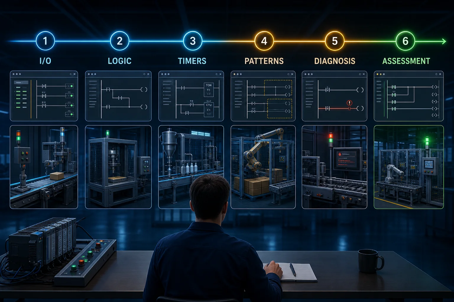
Each course stage adds a specific capability and an observable test. The goal is not to collect lesson views; it is to build, diagnose and prove increasingly realistic PLC behaviour.

Six-stage PLC programming course roadmap from I O and Boolean logic through timers, patterns, diagnosis and practical assessment
01The course moves from observable I/O behaviour to reusable control patterns, fault reasoning and an assessment that produces evidence—not just lesson completion.
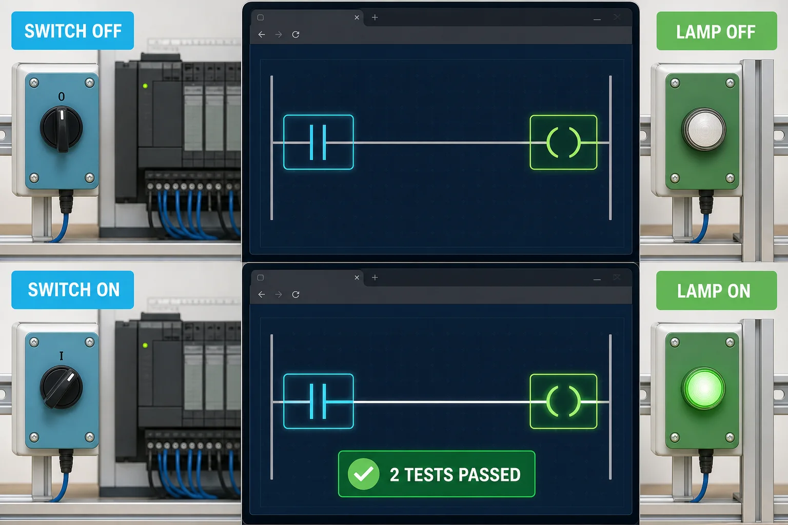
Beginner PLC switch and lamp lesson showing off and on states, matching ladder contact and coil, and two tests passed
02The first learning loop is deliberately small: predict the state, run both input cases and prove that the output follows the program.
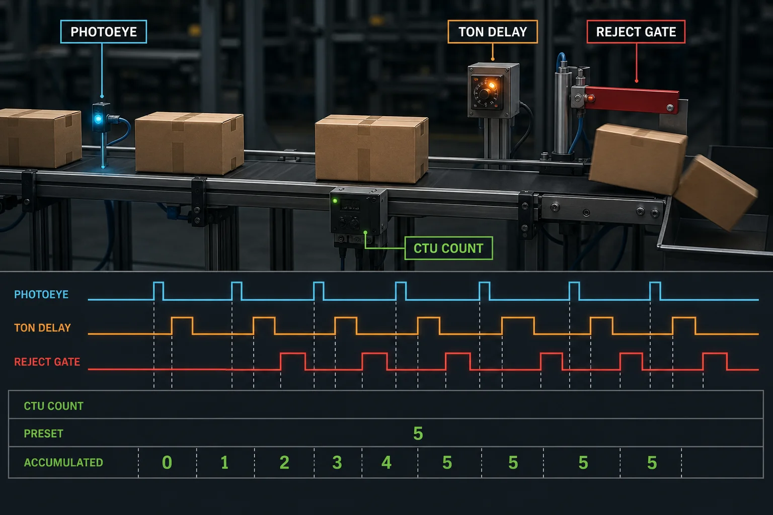
PLC conveyor lesson aligning a photoeye pulse, TON delay, reject gate action and CTU counter accumulator
03Timers and counters become understandable when their internal state is aligned with sensor pulses and visible machine events.
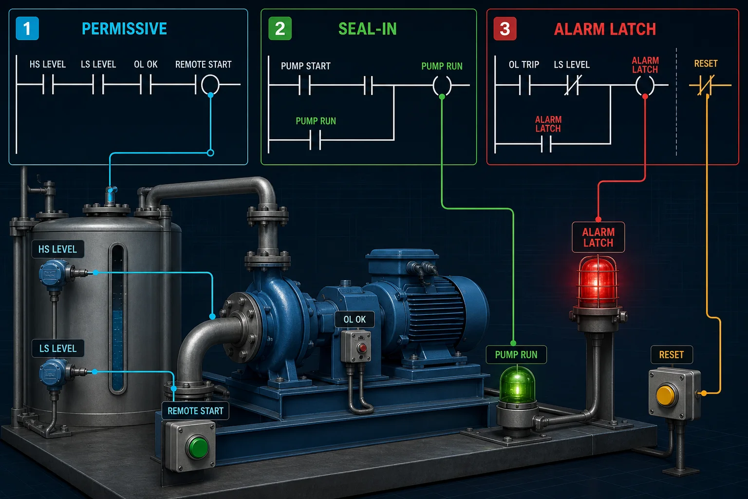
Pump-skid PLC lesson connecting permissive, seal-in and alarm-latch patterns to level switches, overload, pump and reset devices
04Reusable patterns are taught in context: permissives decide whether a start is allowed, seal-in logic remembers run state and alarm latches preserve important faults.
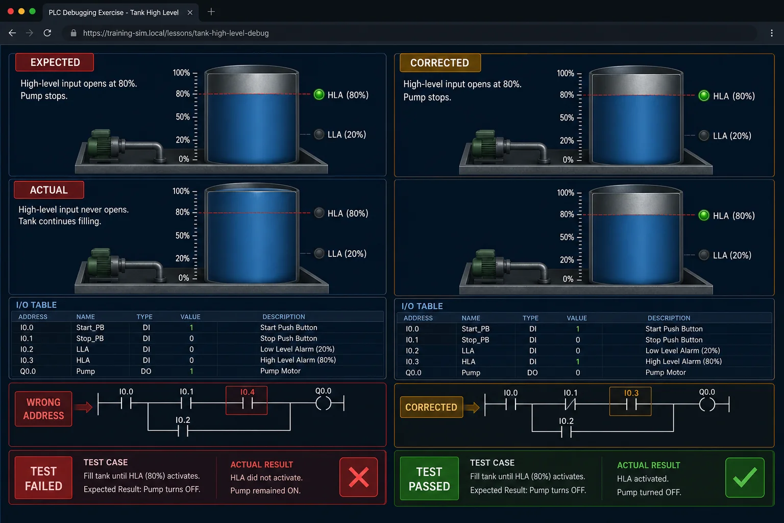
PLC tank debugging exercise comparing expected and actual behaviour, a wrong high-level input address, corrected logic and passing retest
05Debugging starts from a failed requirement. The I/O table and ladder identify the address mismatch; the same test then proves the correction.
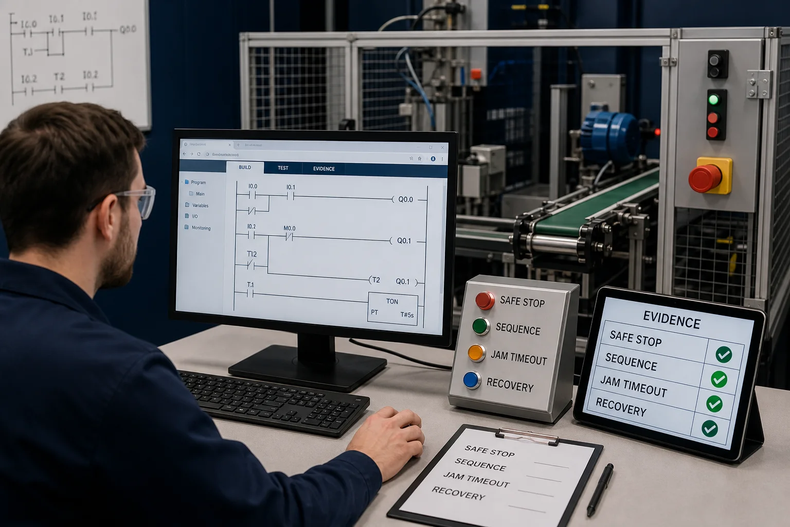
PLC programming practical assessment proving safe stop, sequence, jam timeout and recovery on a guarded conveyor
06A credible assessment asks the learner to interpret requirements, build the control, run hidden cases and preserve evidence for each required behaviour.
Course curriculum

Six modules, structured from first principles.

Work through the modules in order. Each one builds on the last. Resist the urge to jump to the advanced scenarios — the sequencer muscle you build in Module 1 is what makes Module 4 tractable.

PLC programming course — a complete ladder logic rung: input contacts in series and parallel controlling an output coil, read left power rail to rightA basic ladder logic rung between two power rails: an examine-if-closed contact (XIC) in series driving an output coil (OTE).L1L2] [StartXIC I:0/0LampOTE O:0/0
A finished rung — contacts on the left decide whether power flows to the coil on the right. This is what you will be writing by the end of Module 1.

Module 1 — Foundations

The four lessons every PLC programmer must own before writing a single rung. Estimated: 4–8 hours.

  1. 1
    PLC Fundamentals

    What a PLC is, the scan cycle, and how I/O addressing works.

    Read →
  2. 2
    Ladder Logic Basics

    Contacts, coils, XIC/XIO, power flow across a rung.

    Read →
  3. 3
    Latching and Sealing-In

    SET/RESET coils, the seal-in rung, motor start/stop fundamentals.

    Read →
  4. 4
    Timers and Counters

    TON, TOF, TP, CTU, CTD — every beginner trips on timers first.

    Read →
PLC programming course Module 1 — ladder logic symbols: normally-open contact (XIC), normally-closed contact (XIO), and output coil (OTE)The core ladder logic symbols side by side: XIC examine-if-closed, XIO examine-if-open, OTE output energize, OTL output latch and OTU output unlatch.XICIfXIOIfOTEEnergizeLOTLLatchUOTUUnlatch
The three symbols Module 1 starts with — every rung you write is built from contacts and coils.
PLC programming course Module 1 — the seal-in (latching) rung: a START button sets a motor coil that holds itself in until STOP breaks the rungA seal-in latch rung: a Start contact in parallel with a Hold contact, in series with a normally-closed Stop contact, driving an output coil.StartHold (seal)StopMotor
The seal-in rung — the motor start/stop pattern behind your first hands-on exercise.

Module 2 — Logic Building Blocks

Comparisons, math, analog I/O, and Structured Text. Estimated: 4–8 hours.

  1. 5
    Comparisons and Math

    EQU, NEQ, GRT, LES, ADD, SUB — analog thresholds and setpoints.

    Read →
  2. 6
    Function Blocks Advanced

    Advanced timer and counter edge cases; FB instantiation patterns.

    Read →
  3. 7
    Analog I/O and Scaling

    4–20 mA loops, raw counts to engineering units, clamping.

    Read →
  4. 8
    Introduction to Structured Text

    ST syntax, CASE statements, and when to use ST over ladder.

    Read →
PLC programming course Module 2 — on-delay timer (TON): the timer accumulates while its input is true and turns its DONE bit on once the preset time elapsesA TON on-delay timer: the accumulated time bar ramps up toward the preset value, and the done (DN) bit turns on when the accumulator reaches preset.TONPRE 5000ACCACC ramps to PREPREDNdone bit
PLC programming course Module 2 — count-up counter (CTU): each false-to-true input transition increments the accumulator until it reaches the presetA CTU count-up counter: each input pulse increments the accumulator toward the preset, and the done (DN) bit turns on when count reaches preset.count pulsesCTUPRE 5ACC 3ACCcount toward presetDNdone bit
PLC programming course Module 2 — digital and analog I/O: discrete on/off signals plus scaled 4–20 mA analog inputs mapped to engineering unitsA digital input pushbutton wired to a PLC input card, and a PLC output card driving a lamp, with a sinking versus sourcing hint.I/O CARDINPUTOUTPUTPushbuttonI:0/0LampO:0/0sinking (NPN) vs sourcing (PNP)
Module 2 covers analog scaling — turning raw 4–20 mA counts into real engineering units.
PLC programming course Module 2 — Structured Text: an IEC 61131-3 textual language using IF, CASE, and assignment, for logic that is awkward in ladderA small Structured Text code block in an editor: an IF/THEN condition, a TON timer call and assignments, showing text-based PLC programming.main.st — Structured Text1IF Start AND NOT Stop THEN2 Run := TRUE;3END_IF;4DelayTmr(IN := Run, PT := T#5s);5Lamp := DelayTmr.Q;
Structured Text — the IEC 61131-3 textual language you learn alongside ladder in Module 2.

Module 4 — Machine Scenarios

Eight hands-on exercises that run your logic against a simulated machine. Auto-graded. Estimated: 12–24 hours for this module.

The full scenario library contains 140 source-catalogued practice records across motor control, water/HVAC, packaging, safety, and process verticals. Visible availability varies by account, plan, entitlement, and staged rollout.

PLC programming course Module 4 — motor start/stop control: START and STOP push buttons, a holding contact, an overload, and the motor output the simulator runsA 3-wire motor control circuit: Stop and Start pushbuttons, a contactor coil with a seal-in auxiliary contact and an overload contact, driving a motor.StopStartM (seal-in)OLMMmotor
The first scenario you grade — your ladder logic drives this exact motor circuit in the browser simulator.
Who it’s for

Who should take this PLC programming course?

This course is designed for anyone who needs to program PLCs but does not have consistent access to hardware or a structured learning path. Four groups find it particularly useful.

Complete beginners

No programming background needed. The course starts with what a PLC actually is and builds from first principles. You write real ladder logic by lesson two.

Engineering students

Preparing for an internship or controls-engineering interview? The scenario library gives you the practice reps your university lab session could not — without booking lab time.

Maintenance technicians

You already understand the machines. This course bridges the gap from reading ladder logic to writing it — and from recognising a fault to isolating it in code.

Adjacent-field engineers

Mechanical, electrical, or software engineers moving into automation. The scan-cycle model is unlike web or embedded development; the course explains the mental shift explicitly.

Honest comparison

What makes this different from other PLC programming courses?

Most PLC programming classes are video-based. Udemy courses range from $20 to $100 and cover theory well, but you watch a completed rung rather than writing one. If you pause and try to replicate it, you are on your own with no feedback. YouTube tutorials are free but fragmented — there is no guaranteed sequence, no grading, and no way to know when you are ready for the next concept.

Paid platforms like RealPars (approximately $600/year) and PLCacademy (approximately $500 for a full course) are solid and genuinely structured. They are still video-based, and neither ships a browser-based simulator with auto-graded test cases. Classroom training from Allen-Bradley or Siemens partners typically starts at $2,000 per week and requires you to be in a specific city on a specific date.

This course is written, not filmed. Reading a lesson is faster than watching it when you already understand the mechanical context. Every scenario has a test harness: your code either makes the machine behave correctly or it does not, and you get specific feedback about which test case failed. That tight loop — write, run, fail, fix, pass — is the mechanism that builds genuine PLC programming competence faster than passive watching. It is also free to start, with no artificial trial deadline pushing you to rush.

If you want to compare in detail, see our PLC training overview page or how the simulator works.

“A course that cannot fail you cannot teach you. Every scenario here is graded against scripted test cases precisely because ‘watched all the videos’ and ‘can write a working interlock’ are different skills — employers only pay for the second.”
— Paul, author of this course

Whichever course you choose, learn the IEC 61131-3 languages first. The five standard languages — Ladder Diagram, Function Block Diagram, Structured Text, Instruction List, and Sequential Function Chart — are vendor-neutral, so the concepts transfer directly from this simulator to Allen-Bradley Studio 5000, Siemens TIA Portal, CODESYS, or any other platform you meet on the job. You can also dive straight into the learn PLC programming hub if you prefer to follow individual topics rather than the full course track.

PLC programming course — the five IEC 61131-3 languages: Ladder Diagram, Function Block Diagram, Structured Text, Instruction List, and Sequential Function ChartThe five IEC 61131-3 PLC programming languages as chips: Ladder Diagram, Function Block Diagram, Structured Text, Instruction List and Sequential Function Chart.IEC 61131-3 — five languagesLDLadder DiagramFBDFunction BlockSTStructured TextILInstruction ListSFCSequential Func. Chart
The five IEC 61131-3 languages this course is built around — learn these and the skills transfer to any PLC brand.
OptionCostHands-on exercisesAuto-graded
This courseFree (Pro optional)140 source-catalogued practice recordsYes
Udemy video courses$20–100NoneNo
YouTube tutorialsFreeNoneNo
RealPars / PLCacademy~$600/yr (RealPars) / varies (PLCacademy)LimitedNo
Classroom training$2,000+/weekLab time onlyNo
Time commitment

How long does the PLC programming course take?

The short answer: 40–80 hours end to end — roughly 8–16 hours for the fundamentals, 20–40 hours once the machine scenarios are included, and the balance on troubleshooting, safety, and the interview tracks. Evening learners typically finish in six to eight weeks. Set against O*NET’s 2025 median wage of $64,520 for industrial machinery mechanics, the roles this skill most often upgrades, it is a small investment.

Modules 1 and 2 — fundamentals through logic building blocks — take roughly 8–16 hours of focused practice for most learners. By the end you will have written working ladder rungs for timers, counters, seal-in circuits, and Structured Text conditionals. That is the point where you can read someone else’s ladder logic without constantly looking up notation.

Adding the machine scenarios in Modules 3 and 4 brings the total to 20–40 hours. A conveyor sorter, a batch mixer, and a PID temperature loop will each take you two to four hours the first time — longer than they look, because the test harness is precise and your first attempt will miss edge cases you did not think about. That is the point. Missing them in a simulator is free; missing them on a live production line is not.

Completing all six modules and working through the interview prep tracks is a 40–80 hour commitment. Most people doing this in the evenings — one to two hours per night — finish the foundational modules in three to four weeks and reach interview-ready confidence in six to eight weeks. That is a realistic timeline for an entry-level controls-engineering role, not a career change number. [ESTIMATE — based on typical learner progression; individual results vary.]

Explore the full lesson library or go directly to the PLC Fundamentals lesson to start.

Questions

PLC programming course — frequently asked questions.

Yes. A free account includes the first 6 core lessons per dialect and 27 source-tagged free-tier practice records. The /try path guides you through one first program without an account. There is no trial clock and no credit card required to start.

Open Module 1 now.

The PLC Fundamentals lesson takes about 20 minutes to read. The Motor Start/Stop scenario takes about 45 minutes to pass on your first attempt. Both are free.

Also: motor start/stop scenario · traffic light scenario · pricing · about the simulator

Competency and practice field guide

PLC programming course: implementation, evidence and troubleshooting

Direct answer

PLC programming course becomes useful when it connects competencies sequenced from i/o and scan logic to state and diagnostics with lessons, exercises, scenarios and assessments to one skill map, then proves working discrete logic with stop priority and feedback under normal, boundary, fault and recovery conditions. The objective is a repeatable engineering or learning result, not merely activity inside a page or tool.

This guide is written for beginners, technicians and instructors seeking a sequenced route from Boolean logic to tested machine programs. The intended result is specific: the learner can build, test, diagnose and explain a small control system rather than only recall instruction names.

System map / 02

Six concepts that control the result

Treat these as connected checkpoints. Each checkpoint has an expected state, an observable state and a boundary to the next part of the system. That structure prevents a software indication from being mistaken for physical proof.

NODE 01observable

Define the operating contract

competencies sequenced from I/O and scan logic to state and diagnostics. For PLC programming curriculum, record the initial condition, actor, requested change, observable result and stopping condition before selecting a tool or implementation.

NODE 02observable

Map the evidence path

lessons, exercises, scenarios and assessments to one skill map. Separate request, internal state, output or service, physical or user-visible result and independent feedback so each boundary can be inspected.

NODE 03observable

Prove normal operation

working discrete logic with stop priority and feedback. Run more than one cycle from a known state and retain the values, timings or artifacts that demonstrate repeatability.

NODE 04observable

Exercise a boundary case

timing limits, data types, reset and startup behavior. Choose minimum, maximum, simultaneous, delayed or restart conditions that reveal assumptions hidden by the happy path.

NODE 05observable

Diagnose a controlled fault

an injected logic, signal or machine fault. Preserve the first symptom, divide the system at a measurable boundary and change one condition only after predicting the result.

NODE 06observable

Transfer and hand over

course artifacts transferred into a reviewed portfolio. Restore normal state, remove temporary changes, repeat affected checks and document which claims remain limited to the learning environment.

Procedure / 03

A six-step practice and commissioning workflow

Run the steps in order the first time. Later, the same structure becomes a diagnostic loop: define the expected condition, observe the boundary, interpret the difference and choose one proving action.

  1. 01

    Write the acceptance case

    Convert competencies sequenced from i/o and scan logic to state and diagnostics into initial conditions, one stimulus and observable pass criteria.

    Evidence: Another person can repeat the case without guessing the intended result.

    Avoid: Using page completion or an animation as the acceptance criterion.

  2. 02

    Build the map

    Document lessons, exercises, scenarios and assessments to one skill map and name who owns each state or decision.

    Evidence: Every request and result has a source, destination and useful inspection point.

    Avoid: Using the same value as command, status and independent feedback.

  3. 03

    Run the baseline

    Apply working discrete logic with stop priority and feedback from a clean start and record the expected evidence.

    Evidence: Repeated runs produce the same bounded result.

    Avoid: Changing several parameters before a baseline exists.

  4. 04

    Challenge assumptions

    Test timing limits, data types, reset and startup behavior without changing the acceptance contract.

    Evidence: Limits, timing and restart behavior reach defined states.

    Avoid: Testing only one ideal sequence.

  5. 05

    Isolate one failure

    Introduce or analyse an injected logic, signal or machine fault and locate the first disagreement.

    Evidence: The proving action distinguishes the leading hypotheses.

    Avoid: Resetting, forcing or replacing before evidence is retained.

  6. 06

    Close the evidence loop

    Complete course artifacts transferred into a reviewed portfolio and repeat the affected regression cases.

    Evidence: A learner completes the surface by explaining the result, passing a changed case and identifying what still requires supervised target-equipment practice.

    Avoid: Treating an acknowledged message or one successful rerun as handover.

Diagnostic matrix / 04

Symptoms, proving points and next actions

The table is a reasoning aid, not a parts-replacement chart. Preserve the initial symptom, inspect the named boundary and use the interpretation to choose the next controlled test. Site safety procedures and equipment manuals remain authoritative.

Diagnostic symptoms, inspection points, interpretations and next actions for PLC programming course: implementation, evidence and troubleshooting
Observed symptomInspectInterpretationNext proving action
The expected result is unclearRequirement, initial state, actor, stimulus, units and pass conditionThe learner, instructor and assessor may be solving different versions of the task.Rewrite one observable acceptance case before continuing.
Internal state changes but the outcome does notRequest, final owner, output or service boundary and independent feedbackA software or interface indication proves intent at one layer, not the complete outcome.Trace the first boundary after the changing state.
Normal case passes but an edge case failsLimits, timing, simultaneous events, reset and restart assumptionsThe implementation contains a hidden assumption exposed by the changed condition.Add the failed boundary as a permanent regression case.
The failure disappears after resetOriginal symptom, histories, diagnostics, timestamps and active causeReset changed evidence or state without proving the initiating cause.Reproduce under a controlled condition and preserve pre/post-event data.
Simulator and target disagreeModel boundary, software version, task timing, I/O behavior, data types and configurationA learning model and the intended target do not share one of the recorded assumptions.Reduce the case and verify against current target documentation.
The result cannot be explainedPrediction, observation, proving action, alternative hypotheses and limitationsActivity occurred but the evidence is not yet transferable or reviewable.Have the learner defend the signal path and repeat a changed case.

Product evidence / 05

What the browser practice can actually demonstrate

The browser platform can retain programs, scenario results, attempts and observable machine state so practice is attached to evidence rather than seat time alone.

Where simulation stops

Online curriculum cannot replace target-hardware commissioning, safety validation or supervised physical wiring practice.

Commissioning notebook / 06

Six cases that turn the concepts into evidence

Use these as written briefs rather than click-through instructions. For every case, state the expected condition before acting, retain the first useful observation and explain why the final result proves the requirement. A different program or component choice can still be correct when it produces the same bounded behavior and evidence.

Case 01

predict → observe → prove

Prove define the operating contract

Engineering context. competencies sequenced from I/O and scan logic to state and diagnostics. For PLC programming curriculum, record the initial condition, actor, requested change, observable result and stopping condition before selecting a tool or implementation. Begin with a written normal condition and identify which request, state, physical result or communication value will provide independent confirmation. Do not begin by changing the configuration; the initial state is part of the evidence and should remain reproducible.

Controlled setup. Use the “Write the acceptance case” stage of the workflow: convert competencies sequenced from i/o and scan logic to state and diagnostics into initial conditions, one stimulus and observable pass criteria. The acceptance record should show this result: another person can repeat the case without guessing the intended result. Record initial conditions, the exact stimulus and the observation point so another learner can repeat the case without relying on your memory.

Fault challenge. Introduce or analyse “The expected result is unclear” as one bounded deviation. Inspect requirement, initial state, actor, stimulus, units and pass condition The working interpretation is that the learner, instructor and assessor may be solving different versions of the task. The next proving action is to rewrite one observable acceptance case before continuing. Change only one condition before observing the result, and preserve timestamps or measurements where timing matters.

Review and recovery. The most common trap here is using page completion or an animation as the acceptance criterion. After restoring the cause, repeat the normal case and at least one stop, timeout, disconnect or restart boundary relevant to this topic. Remove temporary forces and bypasses, return the model to a known state and retain the evidence that both operation and recovery are deliberate.

Explain it aloud: What should I learn first about PLC programming curriculum? A defensible short answer is: Start with the operating contract and evidence path: competencies sequenced from i/o and scan logic to state and diagnostics, followed by lessons, exercises, scenarios and assessments to one skill map. Add advanced features only after the baseline is predictable.

Case 02

predict → observe → prove

Prove map the evidence path

Engineering context. lessons, exercises, scenarios and assessments to one skill map. Separate request, internal state, output or service, physical or user-visible result and independent feedback so each boundary can be inspected. Begin with a written normal condition and identify which request, state, physical result or communication value will provide independent confirmation. Do not begin by changing the configuration; the initial state is part of the evidence and should remain reproducible.

Controlled setup. Use the “Build the map” stage of the workflow: document lessons, exercises, scenarios and assessments to one skill map and name who owns each state or decision. The acceptance record should show this result: every request and result has a source, destination and useful inspection point. Record initial conditions, the exact stimulus and the observation point so another learner can repeat the case without relying on your memory.

Fault challenge. Introduce or analyse “Internal state changes but the outcome does not” as one bounded deviation. Inspect request, final owner, output or service boundary and independent feedback The working interpretation is that a software or interface indication proves intent at one layer, not the complete outcome. The next proving action is to trace the first boundary after the changing state. Change only one condition before observing the result, and preserve timestamps or measurements where timing matters.

Review and recovery. The most common trap here is using the same value as command, status and independent feedback. After restoring the cause, repeat the normal case and at least one stop, timeout, disconnect or restart boundary relevant to this topic. Remove temporary forces and bypasses, return the model to a known state and retain the evidence that both operation and recovery are deliberate.

Explain it aloud: How do I practise PLC programming curriculum effectively? A defensible short answer is: Use short cases with known initial conditions, a written prediction, one action and an observable result. Then alter a boundary or fault and explain why the evidence changed.

Case 03

predict → observe → prove

Prove prove normal operation

Engineering context. working discrete logic with stop priority and feedback. Run more than one cycle from a known state and retain the values, timings or artifacts that demonstrate repeatability. Begin with a written normal condition and identify which request, state, physical result or communication value will provide independent confirmation. Do not begin by changing the configuration; the initial state is part of the evidence and should remain reproducible.

Controlled setup. Use the “Run the baseline” stage of the workflow: apply working discrete logic with stop priority and feedback from a clean start and record the expected evidence. The acceptance record should show this result: repeated runs produce the same bounded result. Record initial conditions, the exact stimulus and the observation point so another learner can repeat the case without relying on your memory.

Fault challenge. Introduce or analyse “Normal case passes but an edge case fails” as one bounded deviation. Inspect limits, timing, simultaneous events, reset and restart assumptions The working interpretation is that the implementation contains a hidden assumption exposed by the changed condition. The next proving action is to add the failed boundary as a permanent regression case. Change only one condition before observing the result, and preserve timestamps or measurements where timing matters.

Review and recovery. The most common trap here is changing several parameters before a baseline exists. After restoring the cause, repeat the normal case and at least one stop, timeout, disconnect or restart boundary relevant to this topic. Remove temporary forces and bypasses, return the model to a known state and retain the evidence that both operation and recovery are deliberate.

Explain it aloud: What counts as proof of competence? A defensible short answer is: A repeatable artifact or system result plus an explanation of the signal path is stronger than time spent, screenshots or a copied answer. Physical competence requires separate supervised evidence.

Case 04

predict → observe → prove

Prove exercise a boundary case

Engineering context. timing limits, data types, reset and startup behavior. Choose minimum, maximum, simultaneous, delayed or restart conditions that reveal assumptions hidden by the happy path. Begin with a written normal condition and identify which request, state, physical result or communication value will provide independent confirmation. Do not begin by changing the configuration; the initial state is part of the evidence and should remain reproducible.

Controlled setup. Use the “Challenge assumptions” stage of the workflow: test timing limits, data types, reset and startup behavior without changing the acceptance contract. The acceptance record should show this result: limits, timing and restart behavior reach defined states. Record initial conditions, the exact stimulus and the observation point so another learner can repeat the case without relying on your memory.

Fault challenge. Introduce or analyse “The failure disappears after reset” as one bounded deviation. Inspect original symptom, histories, diagnostics, timestamps and active cause The working interpretation is that reset changed evidence or state without proving the initiating cause. The next proving action is to reproduce under a controlled condition and preserve pre/post-event data. Change only one condition before observing the result, and preserve timestamps or measurements where timing matters.

Review and recovery. The most common trap here is testing only one ideal sequence. After restoring the cause, repeat the normal case and at least one stop, timeout, disconnect or restart boundary relevant to this topic. Remove temporary forces and bypasses, return the model to a known state and retain the evidence that both operation and recovery are deliberate.

Explain it aloud: Why test faults and restart behavior? A defensible short answer is: Because an injected logic, signal or machine fault or timing limits, data types, reset and startup behavior can expose assumptions that never appear during ideal startup and steady operation.

Case 05

predict → observe → prove

Prove diagnose a controlled fault

Engineering context. an injected logic, signal or machine fault. Preserve the first symptom, divide the system at a measurable boundary and change one condition only after predicting the result. Begin with a written normal condition and identify which request, state, physical result or communication value will provide independent confirmation. Do not begin by changing the configuration; the initial state is part of the evidence and should remain reproducible.

Controlled setup. Use the “Isolate one failure” stage of the workflow: introduce or analyse an injected logic, signal or machine fault and locate the first disagreement. The acceptance record should show this result: the proving action distinguishes the leading hypotheses. Record initial conditions, the exact stimulus and the observation point so another learner can repeat the case without relying on your memory.

Fault challenge. Introduce or analyse “Simulator and target disagree” as one bounded deviation. Inspect model boundary, software version, task timing, I/O behavior, data types and configuration The working interpretation is that a learning model and the intended target do not share one of the recorded assumptions. The next proving action is to reduce the case and verify against current target documentation. Change only one condition before observing the result, and preserve timestamps or measurements where timing matters.

Review and recovery. The most common trap here is resetting, forcing or replacing before evidence is retained. After restoring the cause, repeat the normal case and at least one stop, timeout, disconnect or restart boundary relevant to this topic. Remove temporary forces and bypasses, return the model to a known state and retain the evidence that both operation and recovery are deliberate.

Explain it aloud: Can browser practice replace official software or hardware? A defensible short answer is: No. It can build concepts and diagnostic reasoning. Exact firmware, I/O electrical behavior, networking, safety and commissioning require current official tools, documentation and target equipment.

Case 06

predict → observe → prove

Prove transfer and hand over

Engineering context. course artifacts transferred into a reviewed portfolio. Restore normal state, remove temporary changes, repeat affected checks and document which claims remain limited to the learning environment. Begin with a written normal condition and identify which request, state, physical result or communication value will provide independent confirmation. Do not begin by changing the configuration; the initial state is part of the evidence and should remain reproducible.

Controlled setup. Use the “Close the evidence loop” stage of the workflow: complete course artifacts transferred into a reviewed portfolio and repeat the affected regression cases. The acceptance record should show this result: a learner completes the surface by explaining the result, passing a changed case and identifying what still requires supervised target-equipment practice. Record initial conditions, the exact stimulus and the observation point so another learner can repeat the case without relying on your memory.

Fault challenge. Introduce or analyse “The result cannot be explained” as one bounded deviation. Inspect prediction, observation, proving action, alternative hypotheses and limitations The working interpretation is that activity occurred but the evidence is not yet transferable or reviewable. The next proving action is to have the learner defend the signal path and repeat a changed case. Change only one condition before observing the result, and preserve timestamps or measurements where timing matters.

Review and recovery. The most common trap here is treating an acknowledged message or one successful rerun as handover. After restoring the cause, repeat the normal case and at least one stop, timeout, disconnect or restart boundary relevant to this topic. Remove temporary forces and bypasses, return the model to a known state and retain the evidence that both operation and recovery are deliberate.

Explain it aloud: How should progress be documented? A defensible short answer is: Keep the requirement, initial state, program or configuration, observed values, fault hypothesis, proving action, recovery result and a concise limitations statement.

Answer surface / 07

Questions people ask about PLC programming course

These concise answers define the operating, training and product boundaries most often missed in broad summaries. The full workflow and diagnostic table above provide the evidence behind them.

What should I learn first about PLC programming curriculum?

Start with the operating contract and evidence path: competencies sequenced from i/o and scan logic to state and diagnostics, followed by lessons, exercises, scenarios and assessments to one skill map. Add advanced features only after the baseline is predictable.

How do I practise PLC programming curriculum effectively?

Use short cases with known initial conditions, a written prediction, one action and an observable result. Then alter a boundary or fault and explain why the evidence changed.

What counts as proof of competence?

A repeatable artifact or system result plus an explanation of the signal path is stronger than time spent, screenshots or a copied answer. Physical competence requires separate supervised evidence.

Why test faults and restart behavior?

Because an injected logic, signal or machine fault or timing limits, data types, reset and startup behavior can expose assumptions that never appear during ideal startup and steady operation.

Can browser practice replace official software or hardware?

No. It can build concepts and diagnostic reasoning. Exact firmware, I/O electrical behavior, networking, safety and commissioning require current official tools, documentation and target equipment.

How should progress be documented?

Keep the requirement, initial state, program or configuration, observed values, fault hypothesis, proving action, recovery result and a concise limitations statement.

What should I do when the answer differs from a guide?

Check assumptions, version, units and initial state first. Reduce the case, compare one boundary at a time and prefer current primary documentation for target-specific behavior.

When is a PLC programming curriculum exercise finished?

A learner completes the surface by explaining the result, passing a changed case and identifying what still requires supervised target-equipment practice.

Real plc programming course footage

See this exact skill in the working simulator.

Watch the real browser product respond to the task on this page, then try the same practical workflow yourself. No slides, concept mockups, install, or credit card.
Try this in the browser
PLC Programming Course — From First Rung to Industrial Scenarios