PLC Simulator
PLC field notesfundamentals

PLC Programming vs Traditional Programming: Python, Arduino & C

How PLC programming differs from Python, C and Arduino: the scan cycle, ladder vs relay logic, determinism, and whether a software dev can make the switch.

PLC Simulation Software9 min read

PLC programming vs traditional programming — scan cycle versus sequential execution

If you write Python, C, or Arduino sketches and you have looked at a PLC program, your first reaction was probably confusion. Where is main()? Why does the whole program look like a wiring diagram? Why are there no while loops driving the logic?

The short version: PLC programming and general-purpose software development solve different problems with different execution models. A PLC is not a slower, weirder microcontroller — it is a machine built around a continuous, deterministic scan cycle that runs your logic from top to bottom, over and over, forever, at a fixed pace. Once that one idea clicks, most of the strangeness disappears.

This post compares PLC programming to the kind of programming you already know, answers the common "vs" questions (PLC vs Python, PLC vs Arduino, ladder vs relay logic), and tells you honestly whether a software developer can pick it up. (If you want the hardware comparison instead — PLC vs a bare microcontroller board — read PLC vs Microcontroller. This post is about the programming paradigm.)

The Core Difference: The Scan Cycle

In a Python script or a C program, execution is sequential and event-driven. You start at an entry point, call functions, block on I/O, wait for events, and the program ends (or sits in an event loop) when there is nothing left to do. Your code controls when things happen.

A PLC works differently. It runs a loop you never write yourself — the scan cycle:

   ┌─────────────────────────────────────────┐
   │  1. READ all physical inputs into memory │
   │  2. SOLVE the entire program top-to-bot  │
   │  3. WRITE the results to physical outputs │
   │  4. Housekeeping / comms / diagnostics    │
   └──────────────────┬──────────────────────┘
                      │  repeat every 1–10 ms
                      └──────────────► (forever)

Every scan, the PLC takes a snapshot of all inputs, evaluates your entire program against that snapshot, and pushes the results to the outputs. Then it does it again. A typical scan is a few milliseconds, and it never stops while the PLC is running.
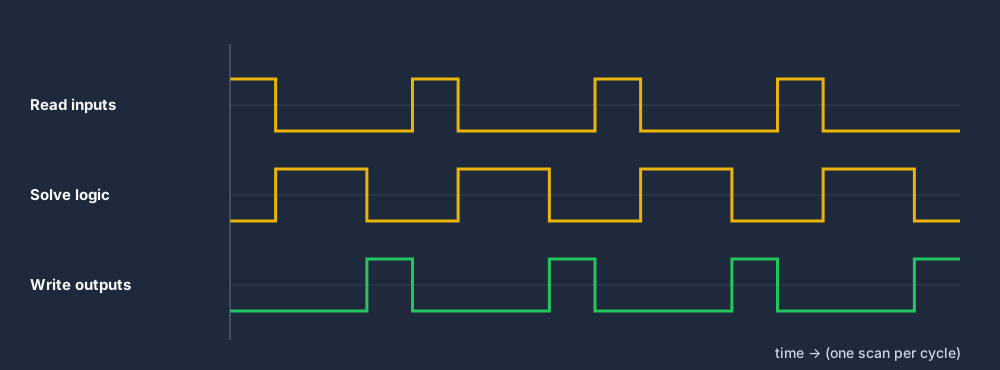
PLC scan cycle timing diagram — inputs read, logic solved, outputs written each cycle

This has consequences that trip up every new developer:

  • You do not write the main loop. Your program is the body that gets re-run each scan. There is no "start" and "end" — there is "what should the outputs be, given the current inputs?"
  • No blocking. You never write sleep(5) or while (sensorOff) {}. Blocking would stall the scan and freeze the whole machine. Delays are done with timer instructions that you check each scan, not by halting execution.
  • Everything appears to run "in parallel." Because the whole program is solved every scan, all your logic is effectively evaluated together, many times per second. You do not schedule tasks; you describe conditions.
  • Inputs are sampled, not interrupt-driven (mostly). Your logic reacts to the input image captured at the top of the scan, which makes timing predictable.

If you are coming from Arduino, the closest analogy is the loop() function — except the PLC's loop is managed by the firmware, guaranteed to run, and instrumented with scan-time monitoring, watchdogs, and I/O image tables you get for free.

For a deeper walk-through, see The PLC Scan Cycle Explained.

Ladder Logic vs Relay Logic

The other thing that looks alien is the language. The most common PLC language, ladder logic (Ladder Diagram), is drawn as rungs of contacts and coils between two vertical rails:

|--[ Start ]--+--[/Stop]--( Motor )--|
|--[ Motor ]--+

This is not decoration. Ladder logic is the software model of physical relay logic — the hard-wired relay panels that PLCs replaced in the 1970s. So "ladder logic vs relay logic" is really one being the digital twin of the other:

  • Relay logic was built from physical relays, contacts, and wires in a control cabinet. To change the behaviour, you rewired the panel.
  • Ladder logic represents those same contacts and coils in software. Current "flows" left-to-right when the series contacts are closed, energising the coil. To change the behaviour, you edit a rung instead of a wire.

The rung above is a classic motor seal-in: press Start and the Motor coil energises; the [ Motor ] contact in the second branch keeps it latched even after you release Start; pressing Stop (a normally-closed contact) breaks the rung and drops it out. An electrician reads that instantly because it maps directly to a wiring diagram they already understand. (More on this pattern in Ladder Logic vs Structured Text.)

That is the deliberate genius of ladder: it let the people who maintained relay panels keep their mental model while gaining the flexibility of software.

PLC Languages vs General-Purpose Languages

PLC languages are standardised under IEC 61131-3, which defines five of them — Ladder Diagram, Structured Text, Function Block Diagram, Sequential Function Chart, and Instruction List. They are domain-specific languages for control, not general-purpose languages.

If you already program, Structured Text is your fastest on-ramp. It is Pascal-like and reads like code:

(* The same motor seal-in, in Structured Text *)
Motor := (Start OR Motor) AND NOT Stop;

But even Structured Text runs inside the scan-cycle model. You are still describing what the outputs should be each scan — you just get IF, CASE, FOR, and real maths to do it. The language changed; the execution model did not.

Side-by-Side Comparison
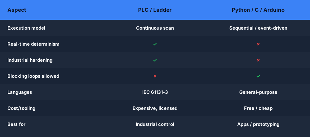
PLC vs Python, C and Arduino comparison table — determinism, execution model and use cases

Reference tableSwipe
PLC ProgrammingTraditional Programming (Python / C / Arduino)
Execution modelContinuous scan cycle (read → solve → write)Sequential / event-driven
Main loopProvided by firmware; you never write itYou write it (or an event loop / framework does)
Blocking & delaysNo blocking; timer instructions checked each scansleep, delay(), blocking I/O all normal
Primary languagesIEC 61131-3 (Ladder, Structured Text, FBD, SFC)Python, C/C++, Java, Rust, etc.
Determinism / real-timeHard real-time, bounded scan timeBest-effort; OS scheduling, GC pauses
HardwareRuggedised, certified, hot-swappable modulesPC, server, dev board, microcontroller
Reliability targetYears of continuous uptime, 24/7 plant runtimeVaries; reboots and crashes tolerated
DebuggingOnline monitoring — watch live values on the rungsBreakpoints, step-through, logs, stack traces
Typical costHundreds to thousands per controller + softwareFree toolchains; commodity hardware
Where it winsMachines, plants, safety, harsh environmentsApps, web, data, prototyping, general compute

Determinism and Real-Time Behaviour

This is the difference that matters most in industry. A PLC guarantees that your logic executes within a bounded, predictable time every single scan. When a guard door opens, the machine must stop within a known number of milliseconds — not "soon," not "after the garbage collector finishes," not "once the OS schedules the thread."

General-purpose stacks make this hard. Python has the GIL and unpredictable garbage-collection pauses. A desktop OS preempts your process whenever it likes. Even C on a PC inherits the operating system's scheduling jitter. You can build real-time systems on general hardware (RTOSes, bare-metal C, real-time Linux), but you have to engineer the determinism yourself. A PLC ships with it.

Reliability and Industrial Hardening

PLCs are built to run for years in places that would destroy a laptop: vibration, dust, temperature swings, electrical noise, and 24/7 duty cycles. They carry certifications (CE, UL, often safety ratings up to SIL/PL levels), tolerate wide voltage ranges, survive surges, and let you hot-swap I/O modules without powering down the line. Downtime on a production line costs real money per minute, so the whole platform is engineered around not failing and being serviceable by a technician at 3 a.m.

Debugging: Online Monitoring vs Breakpoints

In traditional development you set breakpoints, step through code, and read logs. You generally cannot do that to a running machine — halting the CPU would freeze a physical process mid-motion.

Instead, PLC debugging is online monitoring. You connect to the live, running controller and watch values change in real time: contacts light up green as they go true, timer accumulators count, registers update — all without stopping the scan. It is a different muscle, and for many software developers it is the most enjoyable surprise: you can literally see your logic flowing through the rungs while the machine runs.

PLC vs Arduino, Specifically

This comparison comes up constantly, and it deserves a fair answer because Arduino is genuinely great at what it is for.

  • Arduino is a hobby and prototyping platform: an inexpensive microcontroller board you program in C++ via a friendly setup()/loop() IDE. It is perfect for makers, learning electronics, one-off gadgets, and rapid prototyping. It is not industrial-rated — it is not designed for plant-floor noise, it has no certified safety story, no hot-swap I/O, and limited serviceability.
  • A PLC is industrial control hardware: ruggedised, certified, designed for continuous operation, field-wireable to 24 V industrial sensors and actuators, and serviceable by maintenance staff with standard tooling. It costs more because it is built for a context where failure stops production or hurts people.

So the honest framing is not "PLC is better than Arduino." It is: Arduino wins for prototyping, learning, and low-stakes projects; a PLC wins the moment uptime, safety certification, harsh environments, or a maintenance team enters the picture. Plenty of engineers prototype a concept on an Arduino and then implement the real thing on a PLC.

Can a Software Developer Learn PLCs?

Yes — and you are starting from a strong position. You already understand boolean logic, state, conditionals, and data types. Those all transfer.

The single biggest adjustment is the scan-cycle mindset. You have to stop thinking "run this sequence of steps" and start thinking "describe the outputs as a function of the inputs, evaluated continuously." Concretely, that means:

  • Stop reaching for blocking loops and sleep(). Use timers and check them each scan.
  • Stop thinking about when a line runs. The whole program runs every scan; think about conditions, not order of execution.
  • Embrace latching and seal-in patterns instead of imperative state changes.
  • Learn to debug by watching live values, not by stepping through code.

Most developers get comfortable within a couple of weeks of hands-on practice. Start with Structured Text to leverage what you know, then learn ladder logic so you can read the existing programs that fill industry. The career upside is real: controls and automation roles are in demand, often pay well, and value people who can bridge software and the plant floor.

A structured starting point is the Learn PLC Programming path, which takes you from the scan cycle through your first working rungs.

Where Each Paradigm Wins

  • Reach for PLC programming when you are controlling physical machines or processes, when uptime and determinism are non-negotiable, when safety certification is required, or when the environment is harsh and a technician must be able to service it.
  • Reach for traditional programming when you are building software — web apps, data pipelines, services, general compute — or when you are prototyping, where flexibility and a free toolchain matter more than hardened real-time guarantees.

Neither is "more advanced." They are tuned for different worlds. The most valuable engineers in automation are often the ones who understand both.


The fastest way to feel the scan cycle is to write a rung and run it. No install, no credit card. Build real ladder logic against a live machine model right in your browser — and watch the contacts light up as it scans.
Try ladder logic free in your browser →

ShareX / TwitterLinkedIn

From reading to running logic

Practice this yourself in the simulator

Start with guided PLC practice in your browser. No install and no credit card required.

Start practising free

Continue learning

Related field notes

All articles
ladder logic
examples

PLC Programming Examples and Solutions (with Ladder Logic)

Eight classic PLC programming examples with full ladder logic solutions and explanations — motor seal-in, timers, counters, traffic lights, tank control and star-delta.

10 min read
allen bradley
rslogix

RSLogix 500 vs Studio 5000: What's the Difference?

RSLogix 500 programs SLC 500 and MicroLogix; Studio 5000 programs ControlLogix and CompactLogix. Compare hardware, addressing, and which to learn in 2026.

8 min read
ladder logic
function block

Ladder Logic vs Function Block Diagram: When to Use Each

Ladder logic suits discrete interlocks and relay replacement; function block diagram suits analog, PID, and reusable logic. Compare LD vs FBD and pick the right one.

8 min read

Software evaluation field guide

PLC programming versus traditional programming: implementation, evidence and troubleshooting

Direct answer

PLC programming versus traditional programming becomes useful when it connects execution model, task scheduling, physical i/o, persistent state, time, concurrency, failure response, deployment, observability, testing and lifecycle ownership with external condition through sampling or event, program decision, owned state, output or service, feedback and user or process consequence, then proves one bounded control task and one application task specified with equivalent acceptance evidence under normal, boundary, fault and recovery conditions. The objective is a repeatable engineering or learning result, not merely activity inside a page or tool.

This guide is written for software developers, engineering students and PLC beginners translating familiar programming ideas into deterministic machine control. The intended result is specific: the reader can compare execution, state, timing, I/O, failure, deployment and testing without reducing either discipline to syntax.

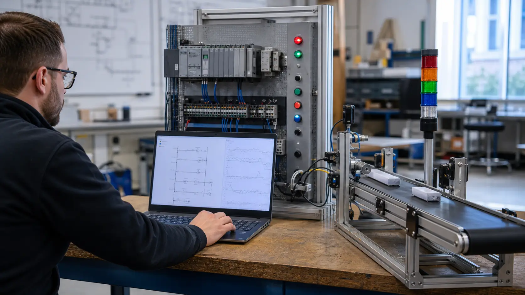
an automation engineer correlating PLC state, scan evidence and a controlled conveyor response at a logic diagnostics workstation while studying cyclic control programming compared with event and application software
The scene keeps cyclic control programming compared with event and application software connected to declared conditions, observable behavior, diagnostic boundaries and evidence that another person can reproduce.

System map / 02

Six concepts that control the result

Treat these as connected checkpoints. Each checkpoint has an expected state, an observable state and a boundary to the next part of the system. That structure prevents a software indication from being mistaken for physical proof.

NODE 01observable

Define the operating contract

execution model, task scheduling, physical I/O, persistent state, time, concurrency, failure response, deployment, observability, testing and lifecycle ownership. For cyclic control programming compared with event and application software, record the initial condition, actor, requested change, observable result and stopping condition before selecting a tool or implementation.

NODE 02observable

Map the evidence path

external condition through sampling or event, program decision, owned state, output or service, feedback and user or process consequence. Separate request, internal state, output or service, physical or user-visible result and independent feedback so each boundary can be inspected.

NODE 03observable

Prove normal operation

one bounded control task and one application task specified with equivalent acceptance evidence. Run more than one cycle from a known state and retain the values, timings or artifacts that demonstrate repeatability.

NODE 04observable

Exercise a boundary case

simultaneous events, delayed input, restart, stale state, communication loss, exception, partial deployment and unavailable dependency. Choose minimum, maximum, simultaneous, delayed or restart conditions that reveal assumptions hidden by the happy path.

NODE 05observable

Diagnose a controlled fault

an execution-model, state, timing, concurrency, interface, deployment, recovery or evidence mismatch. Preserve the first symptom, divide the system at a measurable boundary and change one condition only after predicting the result.

NODE 06observable

Transfer and hand over

the design implemented and tested in the actual runtime with domain-specific safety and operational review. Restore normal state, remove temporary changes, repeat affected checks and document which claims remain limited to the learning environment.

Procedure / 03

A six-step practice and commissioning workflow

Run the steps in order the first time. Later, the same structure becomes a diagnostic loop: define the expected condition, observe the boundary, interpret the difference and choose one proving action.

  1. 01

    Write the acceptance case

    Convert execution model, task scheduling, physical i/o, persistent state, time, concurrency, failure response, deployment, observability, testing and lifecycle ownership into initial conditions, one stimulus and observable pass criteria.

    Evidence: Another person can repeat the case without guessing the intended result.

    Avoid: Using page completion or an animation as the acceptance criterion.

  2. 02

    Build the map

    Document external condition through sampling or event, program decision, owned state, output or service, feedback and user or process consequence and name who owns each state or decision.

    Evidence: Every request and result has a source, destination and useful inspection point.

    Avoid: Using the same value as command, status and independent feedback.

  3. 03

    Run the baseline

    Apply one bounded control task and one application task specified with equivalent acceptance evidence from a clean start and record the expected evidence.

    Evidence: Repeated runs produce the same bounded result.

    Avoid: Changing several parameters before a baseline exists.

  4. 04

    Challenge assumptions

    Test simultaneous events, delayed input, restart, stale state, communication loss, exception, partial deployment and unavailable dependency without changing the acceptance contract.

    Evidence: Limits, timing and restart behavior reach defined states.

    Avoid: Testing only one ideal sequence.

  5. 05

    Isolate one failure

    Introduce or analyse an execution-model, state, timing, concurrency, interface, deployment, recovery or evidence mismatch and locate the first disagreement.

    Evidence: The proving action distinguishes the leading hypotheses.

    Avoid: Resetting, forcing or replacing before evidence is retained.

  6. 06

    Close the evidence loop

    Complete the design implemented and tested in the actual runtime with domain-specific safety and operational review and repeat the affected regression cases.

    Evidence: An evaluation is complete when the same representative job is tested in each candidate and differences are recorded as evidence rather than inferred from feature labels.

    Avoid: Treating an acknowledged message or one successful rerun as handover.

Diagnostic matrix / 04

Symptoms, proving points and next actions

The table is a reasoning aid, not a parts-replacement chart. Preserve the initial symptom, inspect the named boundary and use the interpretation to choose the next controlled test. Site safety procedures and equipment manuals remain authoritative.

Diagnostic symptoms, inspection points, interpretations and next actions for PLC programming versus traditional programming: implementation, evidence and troubleshooting
Observed symptomInspectInterpretationNext proving action
The expected result is unclearRequirement, initial state, actor, stimulus, units and pass conditionThe evaluator, instructor and technical buyer may be solving different versions of the task.Rewrite one observable acceptance case before continuing.
Internal state changes but the outcome does notRequest, final owner, output or service boundary and independent feedbackA software or interface indication proves intent at one layer, not the complete outcome.Trace the first boundary after the changing state.
Normal case passes but an edge case failsLimits, timing, simultaneous events, reset and restart assumptionsThe implementation contains a hidden assumption exposed by the changed condition.Add the failed boundary as a permanent regression case.
The failure disappears after resetOriginal symptom, histories, diagnostics, timestamps and active causeReset changed evidence or state without proving the initiating cause.Reproduce under a controlled condition and preserve pre/post-event data.
Simulator and target disagreeModel boundary, software version, task timing, I/O behavior, data types and configurationA learning model and the intended target do not share one of the recorded assumptions.Reduce the case and verify against current target documentation.
The result cannot be explainedPrediction, observation, proving action, alternative hypotheses and limitationsActivity occurred but the evidence is not yet transferable or reviewable.Have the learner defend the signal path and repeat a changed case.

Product evidence / 05

What the browser practice can actually demonstrate

The public product surface exposes runnable examples, capability boundaries, pricing context and test-harness behavior that can be checked before a purchasing decision.

Where simulation stops

The comparison describes useful engineering patterns, not every PLC runtime, real-time system, application framework or safety lifecycle.

Commissioning notebook / 06

Six cases that turn the concepts into evidence

Use these as written briefs rather than click-through instructions. For every case, state the expected condition before acting, retain the first useful observation and explain why the final result proves the requirement. A different program or component choice can still be correct when it produces the same bounded behavior and evidence.

Case 01

predict → observe → prove

Prove define the operating contract

Engineering context. execution model, task scheduling, physical I/O, persistent state, time, concurrency, failure response, deployment, observability, testing and lifecycle ownership. For cyclic control programming compared with event and application software, record the initial condition, actor, requested change, observable result and stopping condition before selecting a tool or implementation. Begin with a written normal condition and identify which request, state, physical result or communication value will provide independent confirmation. Do not begin by changing the configuration; the initial state is part of the evidence and should remain reproducible.

Controlled setup. Use the “Write the acceptance case” stage of the workflow: convert execution model, task scheduling, physical i/o, persistent state, time, concurrency, failure response, deployment, observability, testing and lifecycle ownership into initial conditions, one stimulus and observable pass criteria. The acceptance record should show this result: another person can repeat the case without guessing the intended result. Record initial conditions, the exact stimulus and the observation point so another learner can repeat the case without relying on your memory.

Fault challenge. Introduce or analyse “The expected result is unclear” as one bounded deviation. Inspect requirement, initial state, actor, stimulus, units and pass condition The working interpretation is that the evaluator, instructor and technical buyer may be solving different versions of the task. The next proving action is to rewrite one observable acceptance case before continuing. Change only one condition before observing the result, and preserve timestamps or measurements where timing matters.

Review and recovery. The most common trap here is using page completion or an animation as the acceptance criterion. After restoring the cause, repeat the normal case and at least one stop, timeout, disconnect or restart boundary relevant to this topic. Remove temporary forces and bypasses, return the model to a known state and retain the evidence that both operation and recovery are deliberate.

Explain it aloud: How is PLC programming different from normal programming? A defensible short answer is: PLC programs commonly execute cyclic tasks against physical I/O and persistent machine state, while application software often responds to events, requests and user workflows. Both require explicit state and testing.

Case 02

predict → observe → prove

Prove map the evidence path

Engineering context. external condition through sampling or event, program decision, owned state, output or service, feedback and user or process consequence. Separate request, internal state, output or service, physical or user-visible result and independent feedback so each boundary can be inspected. Begin with a written normal condition and identify which request, state, physical result or communication value will provide independent confirmation. Do not begin by changing the configuration; the initial state is part of the evidence and should remain reproducible.

Controlled setup. Use the “Build the map” stage of the workflow: document external condition through sampling or event, program decision, owned state, output or service, feedback and user or process consequence and name who owns each state or decision. The acceptance record should show this result: every request and result has a source, destination and useful inspection point. Record initial conditions, the exact stimulus and the observation point so another learner can repeat the case without relying on your memory.

Fault challenge. Introduce or analyse “Internal state changes but the outcome does not” as one bounded deviation. Inspect request, final owner, output or service boundary and independent feedback The working interpretation is that a software or interface indication proves intent at one layer, not the complete outcome. The next proving action is to trace the first boundary after the changing state. Change only one condition before observing the result, and preserve timestamps or measurements where timing matters.

Review and recovery. The most common trap here is using the same value as command, status and independent feedback. After restoring the cause, repeat the normal case and at least one stop, timeout, disconnect or restart boundary relevant to this topic. Remove temporary forces and bypasses, return the model to a known state and retain the evidence that both operation and recovery are deliberate.

Explain it aloud: Is ladder logic easier than traditional code? A defensible short answer is: Its visual conventions can make discrete control paths approachable, but timing, state ownership, abnormal conditions and physical consequences still require disciplined engineering.

Case 03

predict → observe → prove

Prove prove normal operation

Engineering context. one bounded control task and one application task specified with equivalent acceptance evidence. Run more than one cycle from a known state and retain the values, timings or artifacts that demonstrate repeatability. Begin with a written normal condition and identify which request, state, physical result or communication value will provide independent confirmation. Do not begin by changing the configuration; the initial state is part of the evidence and should remain reproducible.

Controlled setup. Use the “Run the baseline” stage of the workflow: apply one bounded control task and one application task specified with equivalent acceptance evidence from a clean start and record the expected evidence. The acceptance record should show this result: repeated runs produce the same bounded result. Record initial conditions, the exact stimulus and the observation point so another learner can repeat the case without relying on your memory.

Fault challenge. Introduce or analyse “Normal case passes but an edge case fails” as one bounded deviation. Inspect limits, timing, simultaneous events, reset and restart assumptions The working interpretation is that the implementation contains a hidden assumption exposed by the changed condition. The next proving action is to add the failed boundary as a permanent regression case. Change only one condition before observing the result, and preserve timestamps or measurements where timing matters.

Review and recovery. The most common trap here is changing several parameters before a baseline exists. After restoring the cause, repeat the normal case and at least one stop, timeout, disconnect or restart boundary relevant to this topic. Remove temporary forces and bypasses, return the model to a known state and retain the evidence that both operation and recovery are deliberate.

Explain it aloud: What should I learn first about cyclic control programming compared with event and application software? A defensible short answer is: Start with the operating contract and evidence path: execution model, task scheduling, physical i/o, persistent state, time, concurrency, failure response, deployment, observability, testing and lifecycle ownership, followed by external condition through sampling or event, program decision, owned state, output or service, feedback and user or process consequence. Add advanced features only after the baseline is predictable.

Case 04

predict → observe → prove

Prove exercise a boundary case

Engineering context. simultaneous events, delayed input, restart, stale state, communication loss, exception, partial deployment and unavailable dependency. Choose minimum, maximum, simultaneous, delayed or restart conditions that reveal assumptions hidden by the happy path. Begin with a written normal condition and identify which request, state, physical result or communication value will provide independent confirmation. Do not begin by changing the configuration; the initial state is part of the evidence and should remain reproducible.

Controlled setup. Use the “Challenge assumptions” stage of the workflow: test simultaneous events, delayed input, restart, stale state, communication loss, exception, partial deployment and unavailable dependency without changing the acceptance contract. The acceptance record should show this result: limits, timing and restart behavior reach defined states. Record initial conditions, the exact stimulus and the observation point so another learner can repeat the case without relying on your memory.

Fault challenge. Introduce or analyse “The failure disappears after reset” as one bounded deviation. Inspect original symptom, histories, diagnostics, timestamps and active cause The working interpretation is that reset changed evidence or state without proving the initiating cause. The next proving action is to reproduce under a controlled condition and preserve pre/post-event data. Change only one condition before observing the result, and preserve timestamps or measurements where timing matters.

Review and recovery. The most common trap here is testing only one ideal sequence. After restoring the cause, repeat the normal case and at least one stop, timeout, disconnect or restart boundary relevant to this topic. Remove temporary forces and bypasses, return the model to a known state and retain the evidence that both operation and recovery are deliberate.

Explain it aloud: How do I practise cyclic control programming compared with event and application software effectively? A defensible short answer is: Use short cases with known initial conditions, a written prediction, one action and an observable result. Then alter a boundary or fault and explain why the evidence changed.

Case 05

predict → observe → prove

Prove diagnose a controlled fault

Engineering context. an execution-model, state, timing, concurrency, interface, deployment, recovery or evidence mismatch. Preserve the first symptom, divide the system at a measurable boundary and change one condition only after predicting the result. Begin with a written normal condition and identify which request, state, physical result or communication value will provide independent confirmation. Do not begin by changing the configuration; the initial state is part of the evidence and should remain reproducible.

Controlled setup. Use the “Isolate one failure” stage of the workflow: introduce or analyse an execution-model, state, timing, concurrency, interface, deployment, recovery or evidence mismatch and locate the first disagreement. The acceptance record should show this result: the proving action distinguishes the leading hypotheses. Record initial conditions, the exact stimulus and the observation point so another learner can repeat the case without relying on your memory.

Fault challenge. Introduce or analyse “Simulator and target disagree” as one bounded deviation. Inspect model boundary, software version, task timing, I/O behavior, data types and configuration The working interpretation is that a learning model and the intended target do not share one of the recorded assumptions. The next proving action is to reduce the case and verify against current target documentation. Change only one condition before observing the result, and preserve timestamps or measurements where timing matters.

Review and recovery. The most common trap here is resetting, forcing or replacing before evidence is retained. After restoring the cause, repeat the normal case and at least one stop, timeout, disconnect or restart boundary relevant to this topic. Remove temporary forces and bypasses, return the model to a known state and retain the evidence that both operation and recovery are deliberate.

Explain it aloud: What counts as proof of competence? A defensible short answer is: A repeatable artifact or system result plus an explanation of the signal path is stronger than time spent, screenshots or a copied answer. Physical competence requires separate supervised evidence.

Case 06

predict → observe → prove

Prove transfer and hand over

Engineering context. the design implemented and tested in the actual runtime with domain-specific safety and operational review. Restore normal state, remove temporary changes, repeat affected checks and document which claims remain limited to the learning environment. Begin with a written normal condition and identify which request, state, physical result or communication value will provide independent confirmation. Do not begin by changing the configuration; the initial state is part of the evidence and should remain reproducible.

Controlled setup. Use the “Close the evidence loop” stage of the workflow: complete the design implemented and tested in the actual runtime with domain-specific safety and operational review and repeat the affected regression cases. The acceptance record should show this result: an evaluation is complete when the same representative job is tested in each candidate and differences are recorded as evidence rather than inferred from feature labels. Record initial conditions, the exact stimulus and the observation point so another learner can repeat the case without relying on your memory.

Fault challenge. Introduce or analyse “The result cannot be explained” as one bounded deviation. Inspect prediction, observation, proving action, alternative hypotheses and limitations The working interpretation is that activity occurred but the evidence is not yet transferable or reviewable. The next proving action is to have the learner defend the signal path and repeat a changed case. Change only one condition before observing the result, and preserve timestamps or measurements where timing matters.

Review and recovery. The most common trap here is treating an acknowledged message or one successful rerun as handover. After restoring the cause, repeat the normal case and at least one stop, timeout, disconnect or restart boundary relevant to this topic. Remove temporary forces and bypasses, return the model to a known state and retain the evidence that both operation and recovery are deliberate.

Explain it aloud: Why test faults and restart behavior? A defensible short answer is: Because an execution-model, state, timing, concurrency, interface, deployment, recovery or evidence mismatch or simultaneous events, delayed input, restart, stale state, communication loss, exception, partial deployment and unavailable dependency can expose assumptions that never appear during ideal startup and steady operation.

Answer surface / 07

Questions people ask about PLC programming versus traditional programming

These concise answers define the operating, training and product boundaries most often missed in broad summaries. The full workflow and diagnostic table above provide the evidence behind them.

How is PLC programming different from normal programming?

PLC programs commonly execute cyclic tasks against physical I/O and persistent machine state, while application software often responds to events, requests and user workflows. Both require explicit state and testing.

Is ladder logic easier than traditional code?

Its visual conventions can make discrete control paths approachable, but timing, state ownership, abnormal conditions and physical consequences still require disciplined engineering.

What should I learn first about cyclic control programming compared with event and application software?

Start with the operating contract and evidence path: execution model, task scheduling, physical i/o, persistent state, time, concurrency, failure response, deployment, observability, testing and lifecycle ownership, followed by external condition through sampling or event, program decision, owned state, output or service, feedback and user or process consequence. Add advanced features only after the baseline is predictable.

How do I practise cyclic control programming compared with event and application software effectively?

Use short cases with known initial conditions, a written prediction, one action and an observable result. Then alter a boundary or fault and explain why the evidence changed.

What counts as proof of competence?

A repeatable artifact or system result plus an explanation of the signal path is stronger than time spent, screenshots or a copied answer. Physical competence requires separate supervised evidence.

Why test faults and restart behavior?

Because an execution-model, state, timing, concurrency, interface, deployment, recovery or evidence mismatch or simultaneous events, delayed input, restart, stale state, communication loss, exception, partial deployment and unavailable dependency can expose assumptions that never appear during ideal startup and steady operation.

Can browser practice replace official software or hardware?

No. It can build concepts and diagnostic reasoning. Exact firmware, I/O electrical behavior, networking, safety and commissioning require current official tools, documentation and target equipment.

How should progress be documented?

Keep the requirement, initial state, program or configuration, observed values, fault hypothesis, proving action, recovery result and a concise limitations statement.