Modbus vs CAN Bus (CANopen): Industrial Protocol vs Embedded Network

TL;DR: Modbus RTU and Modbus TCP are open, register-based polling protocols widely used to connect PLCs to process instruments, drives, and sensors over RS-485 serial or Ethernet. CAN bus is a broadcast, message-based network originally designed for automotive systems; CANopen is the automation profile built on top of it, used primarily in motion control, robotics, and embedded machine networks. Modbus is pulled by a master. CANopen is event-driven and peer-capable. They rarely compete — they serve different machine layers.

Modbus vs CAN Bus — industrial register protocol vs embedded machine network

A controls engineer encounters Modbus when connecting a PLC to a VFD, energy meter, or flow computer. They encounter CANopen when commissioning a servo drive system, a multi-axis robot joint, or a mobile machine hydraulic controller. The two protocols are rarely on the same decision list — but understanding how they differ helps when integrating systems that use both.

Modbus — The Industrial Register Protocol

Modbus was created by Modicon in 1979 for PLC-to-instrument communication. It remains the most widely deployed industrial protocol because it is simple, open, and royalty-free.

Architecture

Modbus is a master/slave (client/server in Modbus TCP) protocol. One master polls one slave at a time. Slaves respond only when addressed. The master controls all communication timing.

Data model

Modbus organises device memory into four tables:

Holding registers (40001–49999): 16-bit read/write — motor speed setpoints, PID setpoints, mode commands.
Input registers (30001–39999): 16-bit read-only — measured process values, fault codes.
Coils (00001–09999): single-bit read/write — start/stop commands.
Discrete inputs (10001–19999): single-bit read-only — limit switches, alarm bits.

Variants

Modbus RTU: binary framing over RS-485 serial bus, up to 247 slaves, 9600–115200 baud.
Modbus TCP: same register model over Ethernet TCP/IP on port 502. Concurrent connections, no baud-rate limit.
Modbus ASCII: printable hex encoding over serial — rarely used in new installations.

CAN Bus and CANopen

CAN (Controller Area Network) was developed by Bosch in the 1980s for automotive wiring harnesses — replacing point-to-point wiring between ECUs. It was later adopted by industrial automation as the physical and data link layer for embedded machine networks.

CAN bus frame

CAN is a broadcast bus. Any node can transmit when the bus is idle. Messages carry an identifier (11-bit standard, 29-bit extended) that defines both the content type and the arbitration priority — lower numeric IDs win bus access over higher IDs without collision.

| Identifier | RTR | DLC | Data (0–8 bytes) | CRC | ACK |

Identifier: message priority and content type — not a device address.
DLC: data length code — number of data bytes in this frame (0–8).
CRC: 15-bit CRC for error detection.
ACK: all receivers acknowledge every valid frame simultaneously — the transmitter knows at least one node received it.

CAN supports multi-master — any node can initiate a message. Arbitration is non-destructive: the node with the lowest-priority ID backs off and retries.

CANopen — the automation profile

CAN defines only the frame format; it says nothing about what the data means. CANopen (CiA 301) is the application-layer profile that maps automation concepts onto CAN frames.

CANopen defines:

PDOs (Process Data Objects): real-time, cyclic or event-driven exchange of I/O data — position, velocity, torque, digital I/O. No handshake, low overhead. Equivalent to Modbus register reads but pushed rather than polled.
SDOs (Service Data Objects): confirmed parameter access — read or write any object dictionary entry. Used for configuration and commissioning (setting acceleration ramps, encoder resolution, current limits). Equivalent to Modbus write register, but with acknowledgement.
NMT (Network Management): start, stop, and reset nodes. A master NMT node controls node state transitions.
Heartbeat / node guarding: node health monitoring — a node broadcasts a heartbeat periodically; if the master misses it, the node is declared failed.
Object Dictionary: every CANopen device has an object dictionary (OD) — a table of parameters (index 0x0000–0xFFFF), each with a data type and access rights. The EDS (Electronic Data Sheet) file describes the OD so a configuration tool can set up the device without knowing it in advance.

CANopen device profiles

CiA publishes device profiles for common equipment:

CiA 402: drives and motion control — servo drives, stepper drives, frequency inverters.
CiA 401: generic I/O modules.
CiA 404: measurement devices.
CiA 417: lift systems.

A servo drive conforming to CiA 402 exposes standardised objects for target position, actual position, control word, and status word — so the PLC motion program works regardless of which brand of drive is installed.

Side-by-Side Comparison

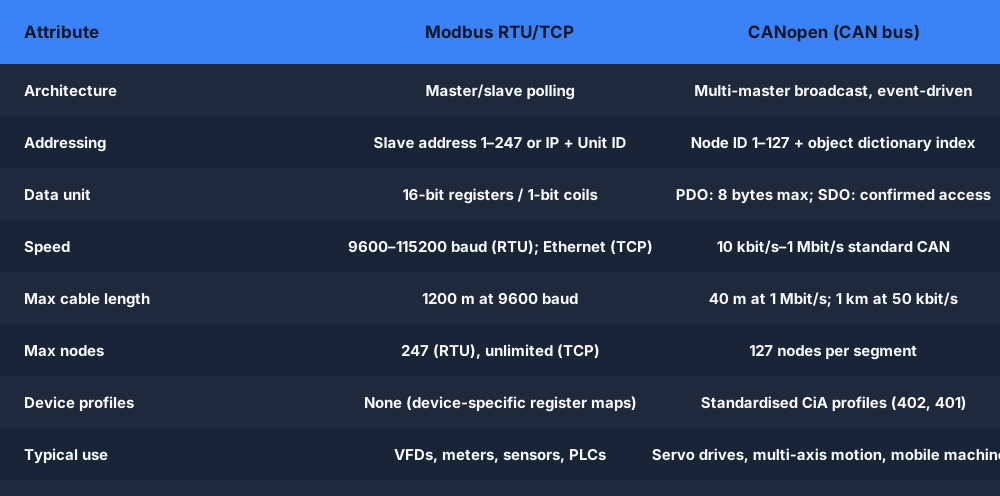
Modbus vs CANopen — frame model, addressing, and application compared

Reference tableSwipe

	Modbus RTU/TCP	CANopen (CAN bus)
Origin	Process automation (1979)	Automotive, then industrial (1993)
Architecture	Master/slave polling	Multi-master broadcast, event-driven
Addressing	Slave address (1–247) or IP + Unit ID	Node ID (1–127) + object dictionary index
Data unit	16-bit registers, 1-bit coils	PDO: up to 8 bytes per frame; SDO: confirmed
Frame size	Variable (function code dependent)	8 bytes max payload per frame
Speed	9600–115200 baud (RTU); 100 Mbit (TCP)	10 kbit/s–1 Mbit/s (standard CAN)
Max cable length	1200 m at 9600 baud	40 m at 1 Mbit/s; 1 km at 50 kbit/s
Max nodes	247 (RTU), unlimited (TCP)	127 nodes per segment
Error handling	CRC; slave returns exception code	15-bit CRC + ACK; hardware error counters
Device profiles	None (register maps are device-specific)	Standardised CiA profiles (402, 401, etc.)
Typical use	VFDs, meters, sensors, PLCs	Servo drives, multi-axis motion, mobile machines

Decision Guide

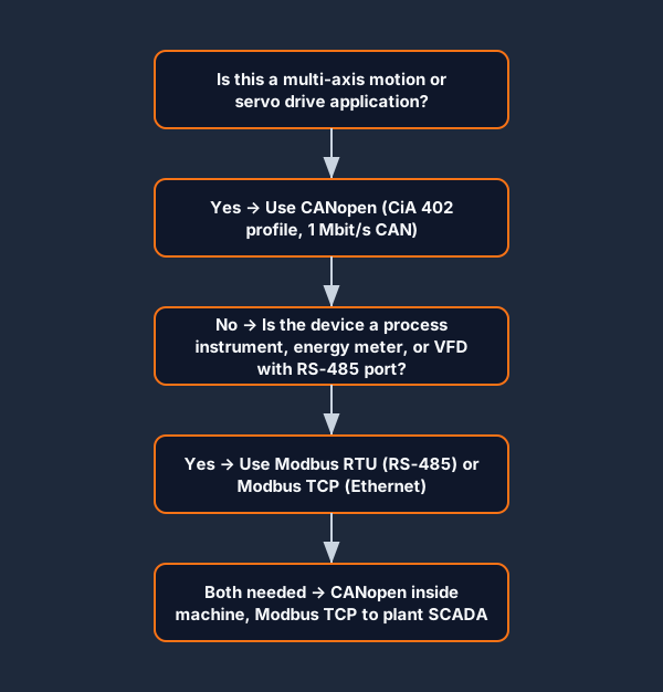
Modbus vs CANopen — which fieldbus fits your application

Use Modbus RTU or TCP when:

Connecting a PLC to process instruments — flow meters, pressure transmitters, energy meters, temperature controllers.
The device's register map is documented and you can poll it.
Cable runs are long (Modbus RTU handles 1200 m).
You need to integrate equipment from many different vendors without a shared device profile.
Your SCADA or PLC natively supports Modbus and does not have a CANopen master module.

Use CANopen when:

Building a machine with multiple motion axes — multi-axis servo, rotary index table, robotic arm.
Your servo drive specifies CiA 402 as its primary interface.
You need synchronised cyclic real-time I/O across multiple nodes (PDO SYNC messaging).
The machine is self-contained and does not need integration into a plant-wide Ethernet network.
You are designing an embedded machine controller (mobile machinery, agricultural equipment, medical devices).

When you need both:

Many industrial machines have both: a CANopen network synchronising servo axes inside the machine enclosure, and a Modbus TCP interface exposing status registers to the plant SCADA. The machine PLC acts as a CANopen master internally and a Modbus TCP server externally.

Frequently Asked Questions

Q: Is CAN bus the same as CANopen?

A: No. CAN bus is the physical and data link layer — the electrical standard and frame format. CANopen is an application-layer protocol built on top of CAN, defining object dictionaries, PDOs, SDOs, NMT, and device profiles. CAN bus also carries other protocols — DeviceNet, J1939, CANaerospace — each with their own application layer.

Q: Can a PLC read a CANopen servo drive?

A: Yes, if the PLC has a CANopen master module or a CANopen fieldbus card. Many PLCs do not include CAN as a standard port — it must be added as an expansion module. Alternatively, some drive manufacturers provide a Modbus TCP or EtherNet/IP gateway above their CANopen internal bus, letting the PLC use standard Ethernet protocols while the drive uses CANopen internally.

Q: What is the speed difference between Modbus and CANopen?

A: At comparable baud rates, CANopen PDOs are faster because they are event-driven — data is pushed when it changes without a request/response cycle. Modbus RTU at 115200 baud can do roughly 200–500 register reads per second; CANopen at 1 Mbit/s with 127 nodes can exchange process data in under 1 ms per cycle for small PDOs. For motion control synchronisation, CANopen is significantly faster.

Q: Is CAN bus still used in industrial automation?

A: Yes, especially in machine building, mobile machinery, medical devices, and robotics. CANopen remains the dominant fieldbus for servo and stepper drives in compact machines. EtherCAT is its successor in high-performance multi-axis motion (microsecond synchronisation), but CANopen at 1 Mbit/s handles most motion applications at lower cost and simpler wiring.

Q: What is DeviceNet and how does it compare to CANopen?

A: DeviceNet is an Allen-Bradley/ODVA protocol that also runs on CAN bus, widely used in North American factory automation. CANopen is the European/international equivalent. Both use CAN as the physical layer but define different object models, device profiles, and network management. DeviceNet is common with Rockwell PLCs; CANopen is common with Siemens, Schneider, and European servo drive manufacturers.

Practise Modbus register reads — the most common way a PLC communicates with a VFD or drive status register — with the Modbus register read scenario. For drive commissioning concepts, the VFD conveyor speed scenario covers frequency reference, run commands, and speed feedback.

Try the Modbus scenario →

ShareX / Twitter LinkedIn

Software evaluation field guide

Modbus versus CAN bus: implementation, evidence and troubleshooting

Direct answer

Modbus versus CAN bus becomes useful when it connects devices, controller, protocol stack, physical layer, topology, distance, bitrate, timing, payload, object model, diagnostics and installed base with application value through register or object definition, message framing, bus access, transport, receiving state and device action, then proves one documented input and output exchange captured with identifiers, values, byte order, timing and healthy diagnostics under normal, boundary, fault and recovery conditions. The objective is a repeatable engineering or learning result, not merely activity inside a page or tool.

This guide is written for controls and embedded engineers comparing an industrial application protocol with a message bus and, where relevant, a higher-layer CANopen device model. The intended result is specific: the reader can separate protocol layer, physical medium, addressing, data model, arbitration, timing, diagnostics and installed-device requirements.

an industrial network engineer tracing PLC, remote I/O, gateway, switch and supervisory-system data evidence while studying Modbus and CAN or CANopen architecture comparison — The physical context keeps Modbus and CAN or CANopen architecture comparison tied to declared inputs, owned decisions, observable results and evidence that another person can verify.

System map / 02

Six concepts that control the result

Treat these as connected checkpoints. Each checkpoint has an expected state, an observable state and a boundary to the next part of the system. That structure prevents a software indication from being mistaken for physical proof.

NODE 01observable

Define the operating contract

devices, controller, protocol stack, physical layer, topology, distance, bitrate, timing, payload, object model, diagnostics and installed base. For Modbus and CAN or CANopen architecture comparison, record the initial condition, actor, requested change, observable result and stopping condition before selecting a tool or implementation.

NODE 02observable

Map the evidence path

application value through register or object definition, message framing, bus access, transport, receiving state and device action. Separate request, internal state, output or service, physical or user-visible result and independent feedback so each boundary can be inspected.

NODE 03observable

Prove normal operation

one documented input and output exchange captured with identifiers, values, byte order, timing and healthy diagnostics. Run more than one cycle from a known state and retain the values, timings or artifacts that demonstrate repeatability.

NODE 04observable

Exercise a boundary case

duplicate identifiers, bus-off, termination, silent node, stale register, endian mismatch, exception response, gateway and restart. Choose minimum, maximum, simultaneous, delayed or restart conditions that reveal assumptions hidden by the happy path.

NODE 05observable

Diagnose a controlled fault

an application-model, mapping, frame, arbitration, timing, physical-layer, configuration or device mismatch. Preserve the first symptom, divide the system at a measurable boundary and change one condition only after predicting the result.

NODE 06observable

Transfer and hand over

the network validated against current protocol and device documentation with captured acceptance evidence. Restore normal state, remove temporary changes, repeat affected checks and document which claims remain limited to the learning environment.

Procedure / 03

A six-step practice and commissioning workflow

Run the steps in order the first time. Later, the same structure becomes a diagnostic loop: define the expected condition, observe the boundary, interpret the difference and choose one proving action.

01
Write the acceptance case
Convert devices, controller, protocol stack, physical layer, topology, distance, bitrate, timing, payload, object model, diagnostics and installed base into initial conditions, one stimulus and observable pass criteria.
Evidence: Another person can repeat the case without guessing the intended result.
Avoid: Using page completion or an animation as the acceptance criterion.
02
Build the map
Document application value through register or object definition, message framing, bus access, transport, receiving state and device action and name who owns each state or decision.
Evidence: Every request and result has a source, destination and useful inspection point.
Avoid: Using the same value as command, status and independent feedback.
03
Run the baseline
Apply one documented input and output exchange captured with identifiers, values, byte order, timing and healthy diagnostics from a clean start and record the expected evidence.
Evidence: Repeated runs produce the same bounded result.
Avoid: Changing several parameters before a baseline exists.
04
Challenge assumptions
Test duplicate identifiers, bus-off, termination, silent node, stale register, endian mismatch, exception response, gateway and restart without changing the acceptance contract.
Evidence: Limits, timing and restart behavior reach defined states.
Avoid: Testing only one ideal sequence.
05
Isolate one failure
Introduce or analyse an application-model, mapping, frame, arbitration, timing, physical-layer, configuration or device mismatch and locate the first disagreement.
Evidence: The proving action distinguishes the leading hypotheses.
Avoid: Resetting, forcing or replacing before evidence is retained.
06
Close the evidence loop
Complete the network validated against current protocol and device documentation with captured acceptance evidence and repeat the affected regression cases.
Evidence: An evaluation is complete when the same representative job is tested in each candidate and differences are recorded as evidence rather than inferred from feature labels.
Avoid: Treating an acknowledged message or one successful rerun as handover.

Diagnostic matrix / 04

Symptoms, proving points and next actions

The table is a reasoning aid, not a parts-replacement chart. Preserve the initial symptom, inspect the named boundary and use the interpretation to choose the next controlled test. Site safety procedures and equipment manuals remain authoritative.

Diagnostic symptoms, inspection points, interpretations and next actions for Modbus versus CAN bus: implementation, evidence and troubleshooting
Observed symptom	Inspect	Interpretation	Next proving action
The expected result is unclear	Requirement, initial state, actor, stimulus, units and pass condition	The evaluator, instructor and technical buyer may be solving different versions of the task.	Rewrite one observable acceptance case before continuing.
Internal state changes but the outcome does not	Request, final owner, output or service boundary and independent feedback	A software or interface indication proves intent at one layer, not the complete outcome.	Trace the first boundary after the changing state.
Normal case passes but an edge case fails	Limits, timing, simultaneous events, reset and restart assumptions	The implementation contains a hidden assumption exposed by the changed condition.	Add the failed boundary as a permanent regression case.
The failure disappears after reset	Original symptom, histories, diagnostics, timestamps and active cause	Reset changed evidence or state without proving the initiating cause.	Reproduce under a controlled condition and preserve pre/post-event data.
Simulator and target disagree	Model boundary, software version, task timing, I/O behavior, data types and configuration	A learning model and the intended target do not share one of the recorded assumptions.	Reduce the case and verify against current target documentation.
The result cannot be explained	Prediction, observation, proving action, alternative hypotheses and limitations	Activity occurred but the evidence is not yet transferable or reviewable.	Have the learner defend the signal path and repeat a changed case.

Product evidence / 05

What the browser practice can actually demonstrate

The public product surface exposes runnable examples, capability boundaries, pricing context and test-harness behavior that can be checked before a purchasing decision.

Where simulation stops

Modbus and raw CAN are not drop-in alternatives at the same layer; CANopen, J1939 and vendor protocols add definitions that raw CAN does not provide.

Commissioning notebook / 06

Six cases that turn the concepts into evidence

Use these as written briefs rather than click-through instructions. For every case, state the expected condition before acting, retain the first useful observation and explain why the final result proves the requirement. A different program or component choice can still be correct when it produces the same bounded behavior and evidence.

Case 01

predict → observe → prove

Prove define the operating contract

Engineering context. devices, controller, protocol stack, physical layer, topology, distance, bitrate, timing, payload, object model, diagnostics and installed base. For Modbus and CAN or CANopen architecture comparison, record the initial condition, actor, requested change, observable result and stopping condition before selecting a tool or implementation. Begin with a written normal condition and identify which request, state, physical result or communication value will provide independent confirmation. Do not begin by changing the configuration; the initial state is part of the evidence and should remain reproducible.

Controlled setup. Use the “Write the acceptance case” stage of the workflow: convert devices, controller, protocol stack, physical layer, topology, distance, bitrate, timing, payload, object model, diagnostics and installed base into initial conditions, one stimulus and observable pass criteria. The acceptance record should show this result: another person can repeat the case without guessing the intended result. Record initial conditions, the exact stimulus and the observation point so another learner can repeat the case without relying on your memory.

Fault challenge. Introduce or analyse “The expected result is unclear” as one bounded deviation. Inspect requirement, initial state, actor, stimulus, units and pass condition The working interpretation is that the evaluator, instructor and technical buyer may be solving different versions of the task. The next proving action is to rewrite one observable acceptance case before continuing. Change only one condition before observing the result, and preserve timestamps or measurements where timing matters.

Review and recovery. The most common trap here is using page completion or an animation as the acceptance criterion. After restoring the cause, repeat the normal case and at least one stop, timeout, disconnect or restart boundary relevant to this topic. Remove temporary forces and bypasses, return the model to a known state and retain the evidence that both operation and recovery are deliberate.

Explain it aloud: Is CAN bus faster than Modbus? A defensible short answer is: The question needs a specific Modbus transport and CAN higher layer. Nominal bitrate alone does not determine application latency, determinism, payload efficiency or device behavior.

Case 02

predict → observe → prove

Prove map the evidence path

Engineering context. application value through register or object definition, message framing, bus access, transport, receiving state and device action. Separate request, internal state, output or service, physical or user-visible result and independent feedback so each boundary can be inspected. Begin with a written normal condition and identify which request, state, physical result or communication value will provide independent confirmation. Do not begin by changing the configuration; the initial state is part of the evidence and should remain reproducible.

Controlled setup. Use the “Build the map” stage of the workflow: document application value through register or object definition, message framing, bus access, transport, receiving state and device action and name who owns each state or decision. The acceptance record should show this result: every request and result has a source, destination and useful inspection point. Record initial conditions, the exact stimulus and the observation point so another learner can repeat the case without relying on your memory.

Fault challenge. Introduce or analyse “Internal state changes but the outcome does not” as one bounded deviation. Inspect request, final owner, output or service boundary and independent feedback The working interpretation is that a software or interface indication proves intent at one layer, not the complete outcome. The next proving action is to trace the first boundary after the changing state. Change only one condition before observing the result, and preserve timestamps or measurements where timing matters.

Review and recovery. The most common trap here is using the same value as command, status and independent feedback. After restoring the cause, repeat the normal case and at least one stop, timeout, disconnect or restart boundary relevant to this topic. Remove temporary forces and bypasses, return the model to a known state and retain the evidence that both operation and recovery are deliberate.

Explain it aloud: What is the difference between CAN and CANopen? A defensible short answer is: CAN defines lower-layer framing and arbitration; CANopen adds device profiles, object dictionaries, network management and communication objects for interoperable automation.

Case 03

predict → observe → prove

Prove prove normal operation

Engineering context. one documented input and output exchange captured with identifiers, values, byte order, timing and healthy diagnostics. Run more than one cycle from a known state and retain the values, timings or artifacts that demonstrate repeatability. Begin with a written normal condition and identify which request, state, physical result or communication value will provide independent confirmation. Do not begin by changing the configuration; the initial state is part of the evidence and should remain reproducible.

Controlled setup. Use the “Run the baseline” stage of the workflow: apply one documented input and output exchange captured with identifiers, values, byte order, timing and healthy diagnostics from a clean start and record the expected evidence. The acceptance record should show this result: repeated runs produce the same bounded result. Record initial conditions, the exact stimulus and the observation point so another learner can repeat the case without relying on your memory.

Fault challenge. Introduce or analyse “Normal case passes but an edge case fails” as one bounded deviation. Inspect limits, timing, simultaneous events, reset and restart assumptions The working interpretation is that the implementation contains a hidden assumption exposed by the changed condition. The next proving action is to add the failed boundary as a permanent regression case. Change only one condition before observing the result, and preserve timestamps or measurements where timing matters.

Review and recovery. The most common trap here is changing several parameters before a baseline exists. After restoring the cause, repeat the normal case and at least one stop, timeout, disconnect or restart boundary relevant to this topic. Remove temporary forces and bypasses, return the model to a known state and retain the evidence that both operation and recovery are deliberate.

Explain it aloud: What should I learn first about Modbus and CAN or CANopen architecture comparison? A defensible short answer is: Start with the operating contract and evidence path: devices, controller, protocol stack, physical layer, topology, distance, bitrate, timing, payload, object model, diagnostics and installed base, followed by application value through register or object definition, message framing, bus access, transport, receiving state and device action. Add advanced features only after the baseline is predictable.

Case 04

predict → observe → prove

Prove exercise a boundary case

Engineering context. duplicate identifiers, bus-off, termination, silent node, stale register, endian mismatch, exception response, gateway and restart. Choose minimum, maximum, simultaneous, delayed or restart conditions that reveal assumptions hidden by the happy path. Begin with a written normal condition and identify which request, state, physical result or communication value will provide independent confirmation. Do not begin by changing the configuration; the initial state is part of the evidence and should remain reproducible.

Controlled setup. Use the “Challenge assumptions” stage of the workflow: test duplicate identifiers, bus-off, termination, silent node, stale register, endian mismatch, exception response, gateway and restart without changing the acceptance contract. The acceptance record should show this result: limits, timing and restart behavior reach defined states. Record initial conditions, the exact stimulus and the observation point so another learner can repeat the case without relying on your memory.

Fault challenge. Introduce or analyse “The failure disappears after reset” as one bounded deviation. Inspect original symptom, histories, diagnostics, timestamps and active cause The working interpretation is that reset changed evidence or state without proving the initiating cause. The next proving action is to reproduce under a controlled condition and preserve pre/post-event data. Change only one condition before observing the result, and preserve timestamps or measurements where timing matters.

Review and recovery. The most common trap here is testing only one ideal sequence. After restoring the cause, repeat the normal case and at least one stop, timeout, disconnect or restart boundary relevant to this topic. Remove temporary forces and bypasses, return the model to a known state and retain the evidence that both operation and recovery are deliberate.

Explain it aloud: How do I practise Modbus and CAN or CANopen architecture comparison effectively? A defensible short answer is: Use short cases with known initial conditions, a written prediction, one action and an observable result. Then alter a boundary or fault and explain why the evidence changed.

Case 05

predict → observe → prove

Prove diagnose a controlled fault

Engineering context. an application-model, mapping, frame, arbitration, timing, physical-layer, configuration or device mismatch. Preserve the first symptom, divide the system at a measurable boundary and change one condition only after predicting the result. Begin with a written normal condition and identify which request, state, physical result or communication value will provide independent confirmation. Do not begin by changing the configuration; the initial state is part of the evidence and should remain reproducible.

Controlled setup. Use the “Isolate one failure” stage of the workflow: introduce or analyse an application-model, mapping, frame, arbitration, timing, physical-layer, configuration or device mismatch and locate the first disagreement. The acceptance record should show this result: the proving action distinguishes the leading hypotheses. Record initial conditions, the exact stimulus and the observation point so another learner can repeat the case without relying on your memory.

Fault challenge. Introduce or analyse “Simulator and target disagree” as one bounded deviation. Inspect model boundary, software version, task timing, I/O behavior, data types and configuration The working interpretation is that a learning model and the intended target do not share one of the recorded assumptions. The next proving action is to reduce the case and verify against current target documentation. Change only one condition before observing the result, and preserve timestamps or measurements where timing matters.

Review and recovery. The most common trap here is resetting, forcing or replacing before evidence is retained. After restoring the cause, repeat the normal case and at least one stop, timeout, disconnect or restart boundary relevant to this topic. Remove temporary forces and bypasses, return the model to a known state and retain the evidence that both operation and recovery are deliberate.

Explain it aloud: What counts as proof of competence? A defensible short answer is: A repeatable artifact or system result plus an explanation of the signal path is stronger than time spent, screenshots or a copied answer. Physical competence requires separate supervised evidence.

Case 06

predict → observe → prove

Prove transfer and hand over

Engineering context. the network validated against current protocol and device documentation with captured acceptance evidence. Restore normal state, remove temporary changes, repeat affected checks and document which claims remain limited to the learning environment. Begin with a written normal condition and identify which request, state, physical result or communication value will provide independent confirmation. Do not begin by changing the configuration; the initial state is part of the evidence and should remain reproducible.

Controlled setup. Use the “Close the evidence loop” stage of the workflow: complete the network validated against current protocol and device documentation with captured acceptance evidence and repeat the affected regression cases. The acceptance record should show this result: an evaluation is complete when the same representative job is tested in each candidate and differences are recorded as evidence rather than inferred from feature labels. Record initial conditions, the exact stimulus and the observation point so another learner can repeat the case without relying on your memory.

Fault challenge. Introduce or analyse “The result cannot be explained” as one bounded deviation. Inspect prediction, observation, proving action, alternative hypotheses and limitations The working interpretation is that activity occurred but the evidence is not yet transferable or reviewable. The next proving action is to have the learner defend the signal path and repeat a changed case. Change only one condition before observing the result, and preserve timestamps or measurements where timing matters.

Review and recovery. The most common trap here is treating an acknowledged message or one successful rerun as handover. After restoring the cause, repeat the normal case and at least one stop, timeout, disconnect or restart boundary relevant to this topic. Remove temporary forces and bypasses, return the model to a known state and retain the evidence that both operation and recovery are deliberate.

Explain it aloud: Why test faults and restart behavior? A defensible short answer is: Because an application-model, mapping, frame, arbitration, timing, physical-layer, configuration or device mismatch or duplicate identifiers, bus-off, termination, silent node, stale register, endian mismatch, exception response, gateway and restart can expose assumptions that never appear during ideal startup and steady operation.

Answer surface / 07

Questions people ask about Modbus versus CAN bus

These concise answers define the operating, training and product boundaries most often missed in broad summaries. The full workflow and diagnostic table above provide the evidence behind them.

Is CAN bus faster than Modbus?

The question needs a specific Modbus transport and CAN higher layer. Nominal bitrate alone does not determine application latency, determinism, payload efficiency or device behavior.

What is the difference between CAN and CANopen?

CAN defines lower-layer framing and arbitration; CANopen adds device profiles, object dictionaries, network management and communication objects for interoperable automation.

What should I learn first about Modbus and CAN or CANopen architecture comparison?

Start with the operating contract and evidence path: devices, controller, protocol stack, physical layer, topology, distance, bitrate, timing, payload, object model, diagnostics and installed base, followed by application value through register or object definition, message framing, bus access, transport, receiving state and device action. Add advanced features only after the baseline is predictable.

How do I practise Modbus and CAN or CANopen architecture comparison effectively?

Use short cases with known initial conditions, a written prediction, one action and an observable result. Then alter a boundary or fault and explain why the evidence changed.

What counts as proof of competence?

A repeatable artifact or system result plus an explanation of the signal path is stronger than time spent, screenshots or a copied answer. Physical competence requires separate supervised evidence.

Why test faults and restart behavior?

Because an application-model, mapping, frame, arbitration, timing, physical-layer, configuration or device mismatch or duplicate identifiers, bus-off, termination, silent node, stale register, endian mismatch, exception response, gateway and restart can expose assumptions that never appear during ideal startup and steady operation.

Can browser practice replace official software or hardware?

No. It can build concepts and diagnostic reasoning. Exact firmware, I/O electrical behavior, networking, safety and commissioning require current official tools, documentation and target equipment.

How should progress be documented?

Keep the requirement, initial state, program or configuration, observed values, fault hypothesis, proving action, recovery result and a concise limitations statement.

Continue the signal path / 08

Related practice and reference pages

Industrial protocols guideContinue from devices, controller, protocol stack, physical layer, topology, distance, bitrate, timing, payload, object model, diagnostics and installed base.Modbus simulatorContinue from application value through register or object definition, message framing, bus access, transport, receiving state and device action.Modbus TCP versus RTUContinue from one documented input and output exchange captured with identifiers, values, byte order, timing and healthy diagnostics.Modbus versus PROFIBUSContinue from duplicate identifiers, bus-off, termination, silent node, stale register, endian mismatch, exception response, gateway and restart.Modbus TCP PLC tutorialContinue from an application-model, mapping, frame, arbitration, timing, physical-layer, configuration or device mismatch.Modbus versus DNP3Continue from the network validated against current protocol and device documentation with captured acceptance evidence.Explore hmi design certificateContinue from devices, controller, protocol stack, physical layer, topology, distance, bitrate, timing, payload, object model, diagnostics and installed base.Motor start-stop PLC scenario field guideContinue from application value through register or object definition, message framing, bus access, transport, receiving state and device action.

Modbus — The Industrial Register Protocol

Architecture

Data model

Variants

CAN Bus and CANopen

CAN bus frame

CANopen — the automation profile

CANopen device profiles

Side-by-Side Comparison

Decision Guide

Frequently Asked Questions

Practice this yourself in the simulator

Related field notes

Modbus TCP vs Modbus RTU: Same Protocol, Different Cables

Modbus vs DNP3: Process Protocol vs Utility Outstation Protocol

PLC Fault Finding: 7 Steps from Symptom to Root Cause

Modbus versus CAN bus: implementation, evidence and troubleshooting

Six concepts that control the result

Define the operating contract

Map the evidence path

Prove normal operation

Exercise a boundary case

Diagnose a controlled fault

Transfer and hand over

A six-step practice and commissioning workflow

Write the acceptance case

Build the map

Run the baseline

Challenge assumptions

Isolate one failure

Close the evidence loop

Symptoms, proving points and next actions

What the browser practice can actually demonstrate

Where simulation stops

Six cases that turn the concepts into evidence

Prove define the operating contract

Prove map the evidence path

Prove prove normal operation

Prove exercise a boundary case

Prove diagnose a controlled fault

Prove transfer and hand over

Questions people ask about Modbus versus CAN bus

Is CAN bus faster than Modbus?

What is the difference between CAN and CANopen?

What should I learn first about Modbus and CAN or CANopen architecture comparison?

How do I practise Modbus and CAN or CANopen architecture comparison effectively?

What counts as proof of competence?

Why test faults and restart behavior?

Can browser practice replace official software or hardware?

How should progress be documented?

Related practice and reference pages

Primary and first-party references

Follow the transaction from wire to register