Free
20 min

Traffic Light PLC Ladder Diagram (Run It Free Online)

A traffic light is the classic first PLC sequencing project: three timed outputs that cycle Green → Yellow → Red forever. Below is the full ladder diagram, the I/O table and the timing chart — and because this is a live scenario, you can write the logic and watch the lights run in your browser without installing anything.

timerssequencesbasics
Traffic Light scenario preview

Ready to build this?

Sign up free — no credit card required. This scenario is included in the free tier.

Sign up to play this scenario →

Already have an account? Log in

Briefing

The finale. Everything you've learned — outputs, NC contacts, AND/OR logic, seal-in, SET/RST, timers — comes together in a 4-way traffic light controller. NS and EW alternate phases. Each green is 10 s, yellow is 3 s, and a 1-second all-red clearance prevents conflicting greens. This is a real control problem — sequence logic, timing, safety. Get it green and you've graduated the PLC-101 curriculum.

Objectives

  • NS green for 10s, then NS yellow for 3s, then NS red
  • EW green for 10s, then EW yellow for 3s, then EW red
  • Only one direction is green or yellow at a time
  • 1-second all-red clearance between direction changes

Hints

  • Use TON timers — one per phase (NS green, NS yellow, all-red, EW green, EW yellow)
  • Chain timers: when TON_NS_G fires (Q=true), start the yellow phase by setting NS_YEL
  • Use a phase variable or SET/RESET coils to track which phase is active

I/O Table

Inputs

POWER_ON

Master power enable

BOOL · %I0.0

Outputs

NS_RED

North-South red lamp

BOOL · %Q0.0

NS_YEL

North-South yellow lamp

BOOL · %Q0.1

NS_GRN

North-South green lamp

BOOL · %Q0.2

EW_RED

East-West red lamp

BOOL · %Q0.3

EW_YEL

East-West yellow lamp

BOOL · %Q0.4

EW_GRN

East-West green lamp

BOOL · %Q0.5

Your program will be tested against:

All test cases run automatically when you submit. Assertions are hidden until you pass.

  1. #1Complete one full cycle

    NS green -> yellow -> red, then EW green -> yellow -> red

  2. #2Never both green simultaneously

    Safety check — conflicting greens would cause collision

How a traffic light PLC program works

A single-direction traffic light needs three digital outputs — Green, Yellow and Red lamps — and a Start input to enable the cycle. The PLC runs three on-delay (TON) timers in a chain so each light is on for a fixed time before handing over to the next.

A typical sequence is Green for 30 seconds, Yellow for 5 seconds, then Red for 35 seconds, after which the cycle repeats. Each timer's done bit both turns off its own light and starts the next light's timer.

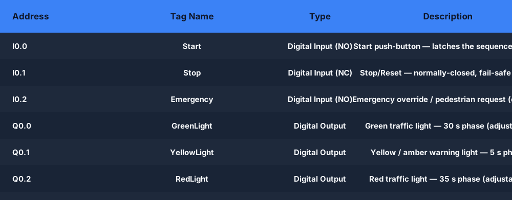
traffic light PLC I/O assignment table inputs outputs
The traffic light I/O: one Start input, three lamp outputs (Green Q0.0, Yellow Q0.1, Red Q0.2).

The traffic light ladder diagram, rung by rung

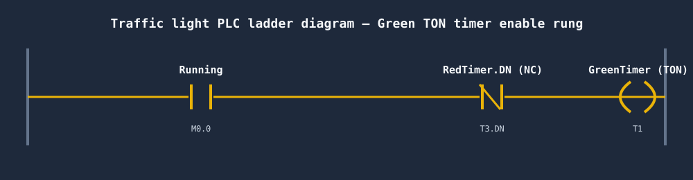
The program is built from three timer rungs that chain together. The Green rung runs its TON while the Red timer is not done; when the Green timer finishes it enables the Yellow timer, and when Yellow finishes it enables the Red timer. When the Red timer finishes the chain resets and Green starts again.

This is the timer-based method — the most common and most readable way to program a traffic light in ladder logic. Each light is driven by the done (.DN) bit of the timer in front of it in the sequence.

traffic light PLC ladder diagram using timers green yellow red
The timer-chained ladder diagram: each TON done bit advances the sequence to the next light.

Traffic light timing sequence diagram

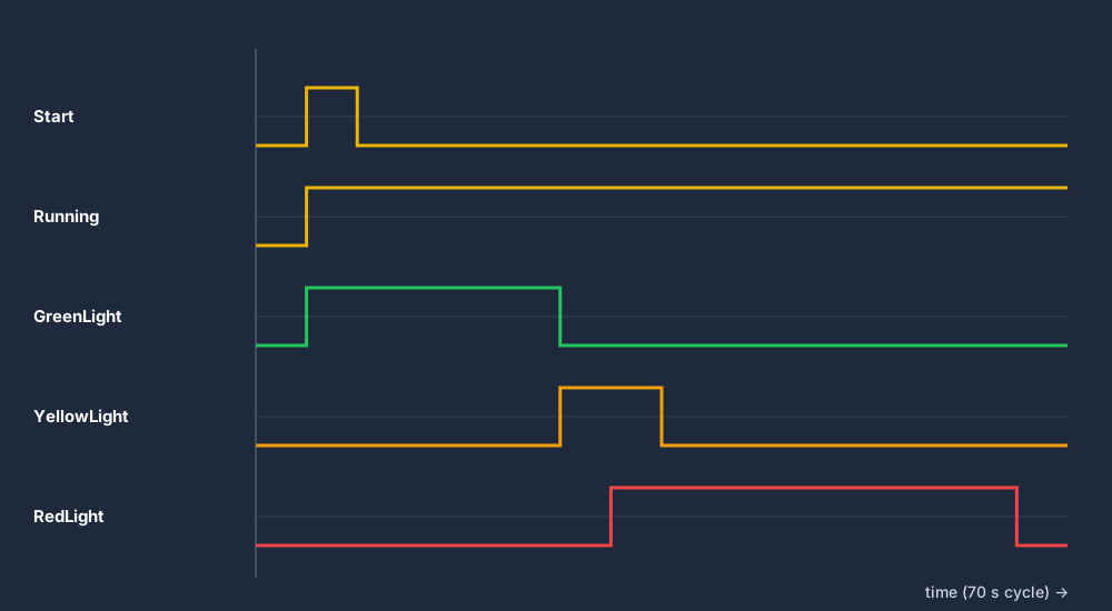
The timing diagram makes the sequence obvious: exactly one lamp output is energised at any moment, and the transitions happen as each timer reaches its preset. Reading the chart top to bottom you can see Green hand over to Yellow, Yellow to Red, and Red back to Green.

When you build this in the simulator, the timing chart is what you are verifying — that the lights never overlap and that each stays on for the right duration.

traffic light PLC program timing sequence diagram green yellow red
One light at a time: the timing chart for the Green → Yellow → Red cycle.

4-way traffic light PLC program

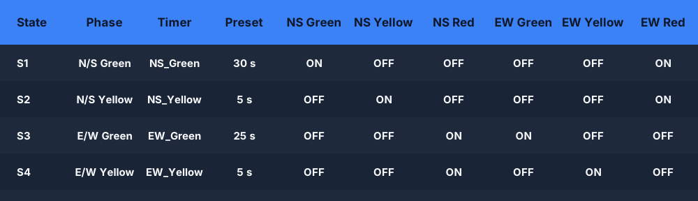
A 4-way intersection adds a second direction (North/South and East/West) that must be interlocked so the two directions are never both green. The cleanest approach is a state machine: each phase (NS green, NS yellow, EW green, EW yellow) is one state, and a master timer steps through them in order.

The state table below shows the four phases and which lamps are energised in each. Because only one phase is active at a time, the cross-direction interlock is automatic.

4 way traffic light PLC ladder diagram state table
The 4-way state table: four phases, North/South and East/West never green together.

Traffic light in Siemens TIA Portal

The logic is identical in Siemens TIA Portal — only the addressing changes. Inputs are %I0.0 style and outputs %Q0.0, and the Siemens TON uses an IEC timer block (with a TIME preset like T#30s) rather than a tag-based timer with a PRE value. The Green/Yellow/Red chain works exactly the same way.

If you learn the sequence here in IEC or Allen-Bradley style, porting it to Siemens is just a matter of swapping the timer block and the I/O addresses.

Troubleshooting your traffic light program

If a light stays on and the sequence never advances, the timer for the next light is not being enabled — check that you are using the previous timer's done bit (.DN), not its timing bit (.TT), to advance the chain.

If a timer never counts, its rung is false: confirm the enabling contact (the Start input on the first rung, or the prior timer's done bit on later rungs) is actually true during the scan.

Traffic light control using PLC — the complete timer-chained program

Traffic light control using a PLC is the textbook way to learn timed sequencing because the whole program is just a chain of on-delay timers feeding each other. The Start input enables the first timer; each timer's done bit turns off its own lamp and starts the next; and when the last timer finishes, the chain wraps around and the cycle repeats forever. There is no operator interaction once it starts — the timers carry the sequence on their own, which is exactly why a traffic light plc program is the classic first project for a new PLC programmer.

Scaling from one direction to a 4 way traffic light plc ladder logic just means treating each intersection phase (NS green, NS yellow, EW green, EW yellow) as one state stepped by a master timer, so the two directions are never green together and the cross-direction interlock is automatic. The whole program is runnable and auto-graded right here in your browser — and to keep a copy of this traffic light PLC ladder diagram (I/O table, single-direction rungs and the 4-way state table) beside you while you build, press Ctrl/Cmd+P on this page and choose Save as PDF.

Frequently asked questions

What PLC instructions are used in a traffic light ladder program?

Three on-delay timers (TON) and their done bits, plus output coils for the Green, Yellow and Red lamps. Each timer's done bit turns off its own light and enables the next timer in the chain.

How do I set the timer presets for a traffic light PLC program?

Set each TON preset to how long that light should stay on — for example Green 30 s, Yellow 5 s, Red 35 s. In Allen-Bradley that is the PRE value; in Siemens it is the IEC timer's TIME preset such as T#30s.

Can I run a traffic light PLC program without hardware?

Yes. This page is a live browser scenario — write the ladder logic, press Run, and watch the lamps cycle on a simulated intersection. No PLC, no install and no licence required.

What is the ladder diagram for a 4-way traffic light using a PLC?

A 4-way intersection is best built as a state machine: one state per phase (North/South green, North/South yellow, East/West green, East/West yellow) stepped by a master timer, so the two directions are never green at the same time.

How does a traffic light PLC program work in Siemens TIA Portal?

Exactly the same logic with Siemens addressing: %I and %Q I/O and IEC TON timer blocks with TIME presets (e.g. T#30s). The Green → Yellow → Red timer chain is identical to the Allen-Bradley or IEC version.

What are the inputs and outputs for a traffic light PLC control system?

A single-direction light needs one input (Start) and three outputs (Green, Yellow, Red lamps). A 4-way intersection doubles the outputs to six lamps across the two directions.

What does a traffic light PLC ladder diagram look like?

A single-direction traffic light PLC ladder diagram is three chained TON timer rungs: the Green rung runs a TON enabled while the Red timer is not done; the Green done bit enables the Yellow TON; the Yellow done bit enables the Red TON; and the Red done bit resets the chain so Green restarts. Each lamp output is driven by the done bit of the timer ahead of it. To keep a copy of this exact ladder diagram, press Ctrl/Cmd+P on this page and choose Save as PDF.

How do you do traffic light control using a PLC?

Traffic light control using a PLC is done with a chain of on-delay (TON) timers: a Start input enables the first timer, each timer's done bit turns off its lamp and starts the next, and the final timer's done bit wraps the chain back to the start so the Green → Yellow → Red cycle repeats indefinitely. Set each timer's preset to that lamp's duration. You can write and run exactly this program in the browser scenario on this page.

What is the 4 way traffic light PLC ladder logic?

A 4 way traffic light PLC ladder logic is best written as a state machine with one state per phase — North/South green, North/South yellow, East/West green, East/West yellow — stepped in order by a master timer. Because only one phase is active at a time, the two directions are never green together and the cross-direction interlock is automatic. The live scenario on this page includes the 4-way state table so you can see which lamps are energised in each phase.

Ready to build this?

Sign up free — no credit card required. This scenario is included in the free tier.

Sign up to play this scenario →

Already have an account? Log in

Runnable simulator field guide

Traffic-light PLC ladder logic: implementation, evidence and troubleshooting

Direct answer

Traffic-light PLC ladder logic becomes useful when it connects approaches, lamp outputs, phase order, duration, all-red clearance, initialization and fault policy with timer and state logic through mutually exclusive lamp commands to visible intersection behavior, then proves multiple complete cycles from a known all-red initial condition under normal, boundary, fault and recovery conditions. The objective is a repeatable engineering or learning result, not merely activity inside a page or tool.

This guide is written for pLC beginners learning states, timers, output exclusivity, clearance intervals, initialization and cyclic sequence tests. The intended result is specific: the learner can implement and explain a deterministic intersection sequence in which conflicting greens never coexist and every transition is testable.

System map / 02

Six concepts that control the result

Treat these as connected checkpoints. Each checkpoint has an expected state, an observable state and a boundary to the next part of the system. That structure prevents a software indication from being mistaken for physical proof.

NODE 01observable

Define the operating contract

approaches, lamp outputs, phase order, duration, all-red clearance, initialization and fault policy. For traffic-light sequence programming, record the initial condition, actor, requested change, observable result and stopping condition before selecting a tool or implementation.

NODE 02observable

Map the evidence path

timer and state logic through mutually exclusive lamp commands to visible intersection behavior. Separate request, internal state, output or service, physical or user-visible result and independent feedback so each boundary can be inspected.

NODE 03observable

Prove normal operation

multiple complete cycles from a known all-red initial condition. Run more than one cycle from a known state and retain the values, timings or artifacts that demonstrate repeatability.

NODE 04observable

Exercise a boundary case

timer boundaries, simultaneous requests, restart mid-phase, stuck output and invalid state. Choose minimum, maximum, simultaneous, delayed or restart conditions that reveal assumptions hidden by the happy path.

NODE 05observable

Diagnose a controlled fault

a transition, timer, latch, output conflict or initialization defect. Preserve the first symptom, divide the system at a measurable boundary and change one condition only after predicting the result.

NODE 06observable

Transfer and hand over

regression evidence for every phase, conflict invariant, stop and restart case. Restore normal state, remove temporary changes, repeat affected checks and document which claims remain limited to the learning environment.

Procedure / 03

A six-step practice and commissioning workflow

Run the steps in order the first time. Later, the same structure becomes a diagnostic loop: define the expected condition, observe the boundary, interpret the difference and choose one proving action.

  1. 01

    Write the acceptance case

    Convert approaches, lamp outputs, phase order, duration, all-red clearance, initialization and fault policy into initial conditions, one stimulus and observable pass criteria.

    Evidence: Another person can repeat the case without guessing the intended result.

    Avoid: Using page completion or an animation as the acceptance criterion.

  2. 02

    Build the map

    Document timer and state logic through mutually exclusive lamp commands to visible intersection behavior and name who owns each state or decision.

    Evidence: Every request and result has a source, destination and useful inspection point.

    Avoid: Using the same value as command, status and independent feedback.

  3. 03

    Run the baseline

    Apply multiple complete cycles from a known all-red initial condition from a clean start and record the expected evidence.

    Evidence: Repeated runs produce the same bounded result.

    Avoid: Changing several parameters before a baseline exists.

  4. 04

    Challenge assumptions

    Test timer boundaries, simultaneous requests, restart mid-phase, stuck output and invalid state without changing the acceptance contract.

    Evidence: Limits, timing and restart behavior reach defined states.

    Avoid: Testing only one ideal sequence.

  5. 05

    Isolate one failure

    Introduce or analyse a transition, timer, latch, output conflict or initialization defect and locate the first disagreement.

    Evidence: The proving action distinguishes the leading hypotheses.

    Avoid: Resetting, forcing or replacing before evidence is retained.

  6. 06

    Close the evidence loop

    Complete regression evidence for every phase, conflict invariant, stop and restart case and repeat the affected regression cases.

    Evidence: A run is complete only when the requested behavior, stop behavior, fault response and recovery are observable from a fresh initial condition.

    Avoid: Treating an acknowledged message or one successful rerun as handover.

Diagnostic matrix / 04

Symptoms, proving points and next actions

The table is a reasoning aid, not a parts-replacement chart. Preserve the initial symptom, inspect the named boundary and use the interpretation to choose the next controlled test. Site safety procedures and equipment manuals remain authoritative.

Diagnostic symptoms, inspection points, interpretations and next actions for Traffic-light PLC ladder logic: implementation, evidence and troubleshooting
Observed symptomInspectInterpretationNext proving action
The expected result is unclearRequirement, initial state, actor, stimulus, units and pass conditionThe operator, programmer and reviewer may be solving different versions of the task.Rewrite one observable acceptance case before continuing.
Internal state changes but the outcome does notRequest, final owner, output or service boundary and independent feedbackA software or interface indication proves intent at one layer, not the complete outcome.Trace the first boundary after the changing state.
Normal case passes but an edge case failsLimits, timing, simultaneous events, reset and restart assumptionsThe implementation contains a hidden assumption exposed by the changed condition.Add the failed boundary as a permanent regression case.
The failure disappears after resetOriginal symptom, histories, diagnostics, timestamps and active causeReset changed evidence or state without proving the initiating cause.Reproduce under a controlled condition and preserve pre/post-event data.
Simulator and target disagreeModel boundary, software version, task timing, I/O behavior, data types and configurationA learning model and the intended target do not share one of the recorded assumptions.Reduce the case and verify against current target documentation.
The result cannot be explainedPrediction, observation, proving action, alternative hypotheses and limitationsActivity occurred but the evidence is not yet transferable or reviewable.Have the learner defend the signal path and repeat a changed case.

Product evidence / 05

What the browser practice can actually demonstrate

The browser runtime joins editable control state to visible I/O and machine or process behavior, allowing the same initial conditions and stimuli to be replayed.

Where simulation stops

The exercise is a learning model, not a road-control design; real traffic systems require applicable standards, certified equipment, fail-safe design and authority approval.

Commissioning notebook / 06

Six cases that turn the concepts into evidence

Use these as written briefs rather than click-through instructions. For every case, state the expected condition before acting, retain the first useful observation and explain why the final result proves the requirement. A different program or component choice can still be correct when it produces the same bounded behavior and evidence.

Case 01

predict → observe → prove

Prove define the operating contract

Engineering context. approaches, lamp outputs, phase order, duration, all-red clearance, initialization and fault policy. For traffic-light sequence programming, record the initial condition, actor, requested change, observable result and stopping condition before selecting a tool or implementation. Begin with a written normal condition and identify which request, state, physical result or communication value will provide independent confirmation. Do not begin by changing the configuration; the initial state is part of the evidence and should remain reproducible.

Controlled setup. Use the “Write the acceptance case” stage of the workflow: convert approaches, lamp outputs, phase order, duration, all-red clearance, initialization and fault policy into initial conditions, one stimulus and observable pass criteria. The acceptance record should show this result: another person can repeat the case without guessing the intended result. Record initial conditions, the exact stimulus and the observation point so another learner can repeat the case without relying on your memory.

Fault challenge. Introduce or analyse “The expected result is unclear” as one bounded deviation. Inspect requirement, initial state, actor, stimulus, units and pass condition The working interpretation is that the operator, programmer and reviewer may be solving different versions of the task. The next proving action is to rewrite one observable acceptance case before continuing. Change only one condition before observing the result, and preserve timestamps or measurements where timing matters.

Review and recovery. The most common trap here is using page completion or an animation as the acceptance criterion. After restoring the cause, repeat the normal case and at least one stop, timeout, disconnect or restart boundary relevant to this topic. Remove temporary forces and bypasses, return the model to a known state and retain the evidence that both operation and recovery are deliberate.

Explain it aloud: What should I learn first about traffic-light sequence programming? A defensible short answer is: Start with the operating contract and evidence path: approaches, lamp outputs, phase order, duration, all-red clearance, initialization and fault policy, followed by timer and state logic through mutually exclusive lamp commands to visible intersection behavior. Add advanced features only after the baseline is predictable.

Case 02

predict → observe → prove

Prove map the evidence path

Engineering context. timer and state logic through mutually exclusive lamp commands to visible intersection behavior. Separate request, internal state, output or service, physical or user-visible result and independent feedback so each boundary can be inspected. Begin with a written normal condition and identify which request, state, physical result or communication value will provide independent confirmation. Do not begin by changing the configuration; the initial state is part of the evidence and should remain reproducible.

Controlled setup. Use the “Build the map” stage of the workflow: document timer and state logic through mutually exclusive lamp commands to visible intersection behavior and name who owns each state or decision. The acceptance record should show this result: every request and result has a source, destination and useful inspection point. Record initial conditions, the exact stimulus and the observation point so another learner can repeat the case without relying on your memory.

Fault challenge. Introduce or analyse “Internal state changes but the outcome does not” as one bounded deviation. Inspect request, final owner, output or service boundary and independent feedback The working interpretation is that a software or interface indication proves intent at one layer, not the complete outcome. The next proving action is to trace the first boundary after the changing state. Change only one condition before observing the result, and preserve timestamps or measurements where timing matters.

Review and recovery. The most common trap here is using the same value as command, status and independent feedback. After restoring the cause, repeat the normal case and at least one stop, timeout, disconnect or restart boundary relevant to this topic. Remove temporary forces and bypasses, return the model to a known state and retain the evidence that both operation and recovery are deliberate.

Explain it aloud: How do I practise traffic-light sequence programming effectively? A defensible short answer is: Use short cases with known initial conditions, a written prediction, one action and an observable result. Then alter a boundary or fault and explain why the evidence changed.

Case 03

predict → observe → prove

Prove prove normal operation

Engineering context. multiple complete cycles from a known all-red initial condition. Run more than one cycle from a known state and retain the values, timings or artifacts that demonstrate repeatability. Begin with a written normal condition and identify which request, state, physical result or communication value will provide independent confirmation. Do not begin by changing the configuration; the initial state is part of the evidence and should remain reproducible.

Controlled setup. Use the “Run the baseline” stage of the workflow: apply multiple complete cycles from a known all-red initial condition from a clean start and record the expected evidence. The acceptance record should show this result: repeated runs produce the same bounded result. Record initial conditions, the exact stimulus and the observation point so another learner can repeat the case without relying on your memory.

Fault challenge. Introduce or analyse “Normal case passes but an edge case fails” as one bounded deviation. Inspect limits, timing, simultaneous events, reset and restart assumptions The working interpretation is that the implementation contains a hidden assumption exposed by the changed condition. The next proving action is to add the failed boundary as a permanent regression case. Change only one condition before observing the result, and preserve timestamps or measurements where timing matters.

Review and recovery. The most common trap here is changing several parameters before a baseline exists. After restoring the cause, repeat the normal case and at least one stop, timeout, disconnect or restart boundary relevant to this topic. Remove temporary forces and bypasses, return the model to a known state and retain the evidence that both operation and recovery are deliberate.

Explain it aloud: What counts as proof of competence? A defensible short answer is: A repeatable artifact or system result plus an explanation of the signal path is stronger than time spent, screenshots or a copied answer. Physical competence requires separate supervised evidence.

Case 04

predict → observe → prove

Prove exercise a boundary case

Engineering context. timer boundaries, simultaneous requests, restart mid-phase, stuck output and invalid state. Choose minimum, maximum, simultaneous, delayed or restart conditions that reveal assumptions hidden by the happy path. Begin with a written normal condition and identify which request, state, physical result or communication value will provide independent confirmation. Do not begin by changing the configuration; the initial state is part of the evidence and should remain reproducible.

Controlled setup. Use the “Challenge assumptions” stage of the workflow: test timer boundaries, simultaneous requests, restart mid-phase, stuck output and invalid state without changing the acceptance contract. The acceptance record should show this result: limits, timing and restart behavior reach defined states. Record initial conditions, the exact stimulus and the observation point so another learner can repeat the case without relying on your memory.

Fault challenge. Introduce or analyse “The failure disappears after reset” as one bounded deviation. Inspect original symptom, histories, diagnostics, timestamps and active cause The working interpretation is that reset changed evidence or state without proving the initiating cause. The next proving action is to reproduce under a controlled condition and preserve pre/post-event data. Change only one condition before observing the result, and preserve timestamps or measurements where timing matters.

Review and recovery. The most common trap here is testing only one ideal sequence. After restoring the cause, repeat the normal case and at least one stop, timeout, disconnect or restart boundary relevant to this topic. Remove temporary forces and bypasses, return the model to a known state and retain the evidence that both operation and recovery are deliberate.

Explain it aloud: Why test faults and restart behavior? A defensible short answer is: Because a transition, timer, latch, output conflict or initialization defect or timer boundaries, simultaneous requests, restart mid-phase, stuck output and invalid state can expose assumptions that never appear during ideal startup and steady operation.

Case 05

predict → observe → prove

Prove diagnose a controlled fault

Engineering context. a transition, timer, latch, output conflict or initialization defect. Preserve the first symptom, divide the system at a measurable boundary and change one condition only after predicting the result. Begin with a written normal condition and identify which request, state, physical result or communication value will provide independent confirmation. Do not begin by changing the configuration; the initial state is part of the evidence and should remain reproducible.

Controlled setup. Use the “Isolate one failure” stage of the workflow: introduce or analyse a transition, timer, latch, output conflict or initialization defect and locate the first disagreement. The acceptance record should show this result: the proving action distinguishes the leading hypotheses. Record initial conditions, the exact stimulus and the observation point so another learner can repeat the case without relying on your memory.

Fault challenge. Introduce or analyse “Simulator and target disagree” as one bounded deviation. Inspect model boundary, software version, task timing, I/O behavior, data types and configuration The working interpretation is that a learning model and the intended target do not share one of the recorded assumptions. The next proving action is to reduce the case and verify against current target documentation. Change only one condition before observing the result, and preserve timestamps or measurements where timing matters.

Review and recovery. The most common trap here is resetting, forcing or replacing before evidence is retained. After restoring the cause, repeat the normal case and at least one stop, timeout, disconnect or restart boundary relevant to this topic. Remove temporary forces and bypasses, return the model to a known state and retain the evidence that both operation and recovery are deliberate.

Explain it aloud: Can browser practice replace official software or hardware? A defensible short answer is: No. It can build concepts and diagnostic reasoning. Exact firmware, I/O electrical behavior, networking, safety and commissioning require current official tools, documentation and target equipment.

Case 06

predict → observe → prove

Prove transfer and hand over

Engineering context. regression evidence for every phase, conflict invariant, stop and restart case. Restore normal state, remove temporary changes, repeat affected checks and document which claims remain limited to the learning environment. Begin with a written normal condition and identify which request, state, physical result or communication value will provide independent confirmation. Do not begin by changing the configuration; the initial state is part of the evidence and should remain reproducible.

Controlled setup. Use the “Close the evidence loop” stage of the workflow: complete regression evidence for every phase, conflict invariant, stop and restart case and repeat the affected regression cases. The acceptance record should show this result: a run is complete only when the requested behavior, stop behavior, fault response and recovery are observable from a fresh initial condition. Record initial conditions, the exact stimulus and the observation point so another learner can repeat the case without relying on your memory.

Fault challenge. Introduce or analyse “The result cannot be explained” as one bounded deviation. Inspect prediction, observation, proving action, alternative hypotheses and limitations The working interpretation is that activity occurred but the evidence is not yet transferable or reviewable. The next proving action is to have the learner defend the signal path and repeat a changed case. Change only one condition before observing the result, and preserve timestamps or measurements where timing matters.

Review and recovery. The most common trap here is treating an acknowledged message or one successful rerun as handover. After restoring the cause, repeat the normal case and at least one stop, timeout, disconnect or restart boundary relevant to this topic. Remove temporary forces and bypasses, return the model to a known state and retain the evidence that both operation and recovery are deliberate.

Explain it aloud: How should progress be documented? A defensible short answer is: Keep the requirement, initial state, program or configuration, observed values, fault hypothesis, proving action, recovery result and a concise limitations statement.

Answer surface / 07

Questions people ask about Traffic-light PLC ladder logic

These concise answers define the operating, training and product boundaries most often missed in broad summaries. The full workflow and diagnostic table above provide the evidence behind them.

What should I learn first about traffic-light sequence programming?

Start with the operating contract and evidence path: approaches, lamp outputs, phase order, duration, all-red clearance, initialization and fault policy, followed by timer and state logic through mutually exclusive lamp commands to visible intersection behavior. Add advanced features only after the baseline is predictable.

How do I practise traffic-light sequence programming effectively?

Use short cases with known initial conditions, a written prediction, one action and an observable result. Then alter a boundary or fault and explain why the evidence changed.

What counts as proof of competence?

A repeatable artifact or system result plus an explanation of the signal path is stronger than time spent, screenshots or a copied answer. Physical competence requires separate supervised evidence.

Why test faults and restart behavior?

Because a transition, timer, latch, output conflict or initialization defect or timer boundaries, simultaneous requests, restart mid-phase, stuck output and invalid state can expose assumptions that never appear during ideal startup and steady operation.

Can browser practice replace official software or hardware?

No. It can build concepts and diagnostic reasoning. Exact firmware, I/O electrical behavior, networking, safety and commissioning require current official tools, documentation and target equipment.

How should progress be documented?

Keep the requirement, initial state, program or configuration, observed values, fault hypothesis, proving action, recovery result and a concise limitations statement.

What should I do when the answer differs from a guide?

Check assumptions, version, units and initial state first. Reduce the case, compare one boundary at a time and prefer current primary documentation for target-specific behavior.

When is a traffic-light sequence programming exercise finished?

A run is complete only when the requested behavior, stop behavior, fault response and recovery are observable from a fresh initial condition.

Real plc traffic light ladder logic footage

See this exact skill in the working simulator.

Watch the real browser product respond to the task on this page, then try the same practical workflow yourself. No slides, concept mockups, install, or credit card.

Try this in the browser
PLC Traffic Light Sequence — Timers and Safe State Changes