PLC Simulator
PLC field notestroubleshooting

PLC Fault Finding: 7 Steps from Symptom to Root Cause

A systematic 7-step PLC fault-finding method covering multimeter discipline, the half-split method, and how to navigate every fault family — from wiring opens to scan-order bugs. Links to live fault scenarios and wiring fault labs.

PLC Simulation Software10 min read

TL;DR: PLC faults fall into four families — wiring, configuration, logic, and intermittent. A systematic 7-step method (define symptom → confirm power → read the ladder → check inputs → trace field wiring → check outputs → verify fix) eliminates random probing and finds root cause in the fewest steps. Multimeter discipline and the half-split method do the heavy lifting. Practising on live fault scenarios before arriving at a real machine dramatically shortens your first-time diagnosis.

PLC fault finding — multimeter discipline and the half-split method

Every experienced controls technician has stood in front of a machine that should be running and isn't. The new technician starts poking randomly. The experienced one pauses, defines the symptom precisely, checks the power supply, reads the ladder, and finds the fault in eight minutes. The difference is not talent — it is method.

This guide covers the full systematic approach: the four fault families, the 7-step method, multimeter discipline, and the half-split technique that halves the fault window at every step.

The Four Fault Families

Before any diagnosis, you need a mental map of where PLC faults live. There are four families. Your job is to identify which family you are in, then apply the correct test procedure for that family.

PLC fault families — wiring, config, logic, intermittent mapped to symptoms, first checks, and tools

Reference tableSwipe
Fault familyTypical symptomFirst checkTool
Wiring faultInput never changes state despite field device operatingSupply voltage at device, then continuity back to cardMultimeter
Configuration faultInput changes but PLC ignores it, or wrong valueVerify tag address, I/O card slot, scaling in softwareSoftware monitor
Logic faultRung stays false even when all inputs appear correctContact types (XIC/XIO), interlock conditions, coil addressLadder monitor
Intermittent faultFault clears itself, reappears under load or heatConnector seating, shielding, data logging over timeMultimeter + data log

The majority of field faults are wiring faults. That is the family to eliminate first.

The 7-Step Method

The 7-step method is the structured path from symptom to root cause. Every step eliminates a portion of the fault window. Skip a step and you risk missing the fault or replacing parts unnecessarily.

Step 1: Define the symptom precisely

Write it down before touching anything. "Motor does not start" is a symptom. "I think the proximity sensor is bad" is a hypothesis — write that separately. You need the symptom isolated before you start forming hypotheses, or you will confirm the hypothesis you already believe instead of finding the actual fault.

Good symptom definitions:

  • "Conveyor does not start when operator presses Start button"
  • "Motor trips on overload within 30 seconds of start, no load"
  • "Output Q0.3 energises but the contactor does not pull in"

Step 2: Confirm power — PLC running, I/O powered, no fault lights

Before reading any ladder logic, confirm the system is actually powered and healthy. Check:

  • PLC RUN LED is green (or equivalent healthy state)
  • I/O cards have their power LEDs lit
  • No fault/error LEDs are active on the processor or cards
  • Supply voltage at the 24 VDC or mains distribution point is within tolerance

A PLC in fault mode, or a card with a blown supply fuse, will show symptoms that look identical to logic or wiring problems. Eliminate the power layer before moving on.

Step 3: Read the ladder — find the output that should be ON

Open the online ladder monitor and find the output coil for the device that is not operating. Look at the entire rung. Which contact in the rung is false when it should be true? That false contact is your fault target.

In a well-structured program, the output coil name tells you exactly what is supposed to happen. Follow the rung from left rail to right until you find the break in power flow.

Step 4: Check inputs at the I/O card

For the false contact you identified in Step 3:

  1. Check the input LED on the physical I/O card for that channel — is it lit?
  2. Compare the LED state to the tag state in the ladder monitor.

Two scenarios:

  • LED is off, tag is false: The problem is in the field — the field device or its wiring is not delivering the signal. Move to Step 6.
  • LED is on, tag is false: The problem is in software — wrong tag address, card addressing mismatch, or a configuration fault. Check the I/O tree in the software and verify the correct input channel is mapped to the correct tag.

Step 5: Trace field wiring from card to device

Now you are in the wiring layer. Use the half-split method (described below) to find the break.

Start by measuring voltage at the I/O card terminal. If no voltage is present, the supply or return is broken. If voltage is present at the card but the LED is not lit, the card input itself may be suspect — but check the common return before condemning the card.

Work backwards from the card toward the field device. Each measurement halves the remaining fault window.

Step 6: Check the output card and field actuator

If you have reached this step, the input chain is healthy and the logic says the output should be ON. Now check the output side:

  1. Is the output card LED lit for that channel?
    • LED lit but actuator not responding: the problem is in the wiring from the card to the actuator, or in the actuator itself.
    • LED not lit but tag is true: the output card or its fuse has failed.
  2. Measure voltage at the actuator terminals while the output is commanded ON.
    • Correct voltage present, actuator not moving: the actuator is the fault.
    • No voltage at actuator terminals: trace back along the output wiring to find the break.

Step 7: Apply the fix and verify

Make the minimum change needed to address the root cause. Then:

  1. Clear any test forces you applied during diagnosis.
  2. Cycle the machine through a full operational sequence.
  3. Confirm the original symptom is gone.
  4. Confirm no new symptoms have appeared.
  5. Document the fault, root cause, and fix in the maintenance log.

Step 7 is frequently skipped. A machine that starts after a fix is not the same as a machine that has been verified. Verify before you close the job.

Multimeter Discipline

A multimeter is the primary diagnostic tool for wiring faults. Used incorrectly it gives misleading readings. Used correctly it finds any wiring fault in a few measurements.
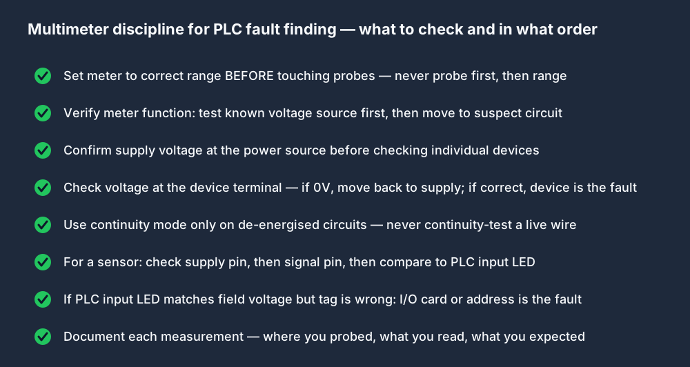
Multimeter discipline for PLC fault finding — correct sequence, what to check and in what order

The correct sequence:

  1. Set the range before probing — never probe first and then range. An auto-ranging meter on a live 415 V circuit takes a fraction of a second to settle. In that time you can misread a voltage that will mislead your diagnosis.
  2. Verify the meter first — test the meter on a known voltage source before moving to the suspect circuit. Dead batteries cause the meter to read low. A faulty lead causes floating readings.
  3. Confirm supply voltage at the source — before probing individual devices, confirm the supply rail is at the correct voltage. A 24 VDC supply sagging to 18 V explains everything.
  4. Measure at the device terminal — if the device terminal reads the correct voltage and the device is not responding, the device is the fault. If the terminal reads 0 V, the supply side has a break.
  5. Use continuity mode only on de-energised circuits — continuity mode sends a small test current. On a live circuit, other voltage sources confuse the reading and you risk a short. Always de-energise before using continuity.
  6. For a sensor: check supply pin, then signal pin — brown (+24 V), blue (0 V), black (signal). If brown and blue are correct but black never switches, the sensor is faulty or its sensing face is obstructed.
  7. Document every reading — write down where you probed, what you expected, and what you measured. If the fault is intermittent, the log becomes your evidence.

The Half-Split Method

The half-split method is binary search applied to a control circuit. Instead of testing each component sequentially from one end, you start at the midpoint of the circuit and eliminate half the remaining fault window with each measurement.
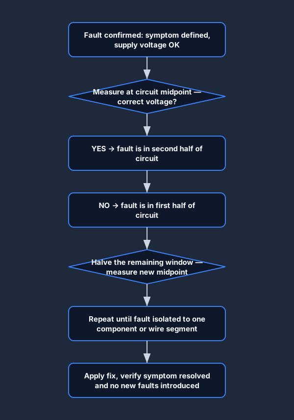
Half-split fault-finding method — binary search through a control circuit, step by step

For a circuit from supply through fuse → OL contact → coil → return:

  1. Measure at the midpoint: the OL contact output.
    • Correct voltage: the fault is between the OL contact and the coil (second half).
    • Zero volts: the fault is between the supply and the OL contact (first half).
  2. Measure at the midpoint of the confirmed half.
  3. Repeat until isolated to a single component.

A 16-component circuit has at most 4 measurements to isolation with half-split, versus up to 16 measurements testing sequentially. For intermittent faults where you have limited time in the fault state, speed matters enormously.

The midpoint of a PLC control circuit is almost always the boundary between the field side and the I/O card. Starting there immediately identifies whether the fault is in the field or in the PLC system — the most useful split available.

Handling Intermittent Faults

Intermittent faults are the hardest to diagnose because the fault clears itself before you can isolate it. Four approaches work:

Data logging: Configure the PLC to log the timestamp and state of the suspect input or output to a data file or historian. When the fault reappears, the log shows you exactly what changed and in what sequence.

Force the fault condition: If you know the conditions that trigger the fault (high ambient temperature, specific machine position, high load), recreate those conditions deliberately and run through your half-split.

Vibration test: Many intermittent faults are loose connections or cracked solder joints that only open under vibration. With the system safely powered down, apply mechanical vibration to suspect cables and connectors while monitoring continuity.

Environmental correlation: Log fault timestamps against shift start times, ambient temperature readings, and machine cycle counts. Patterns like "always after 2 hours of runtime" or "always in the first 10 minutes of a shift in winter" point to thermal or condensation causes.

Applying the Method to the Four Fault Families

Wiring fault: Enter at Step 5. Confirm supply voltage first, then half-split from the I/O card boundary toward the field device. Multimeter in voltage mode throughout.

Configuration fault: Enter at Step 4. The input LED and the tag state disagree. Check the I/O configuration tree — verify channel assignment, card slot addressing, scaling, and tag cross-reference. No multimeter needed.

Logic fault: Enter at Step 3. The inputs are correct but the rung is false. Force each suspect input in the online monitor and watch power flow through the rung. A forced input that does not energise the rung confirms that contact is the problem. Check contact type (XIC vs XIO), the correct tag name, and whether an interlock condition upstream in a different rung has suppressed the permissive.

Intermittent fault: Start with data logging before any hands-on diagnosis. You need evidence of what happened and when before you can half-split anything.

What Needs a Real Meter

A browser simulator — including ours — cannot replace hands-on experience with a real multimeter and a live panel. Here is what you genuinely need real hardware to learn:

  • Developing the muscle memory of safe probe placement on live terminals
  • Recognising the physical signs of a loose connector or burned contact
  • Understanding the feeling of a high-resistance connection versus a good one
  • Correctly identifying polarity, phase, and common returns by sight in a real wiring arrangement
  • Responding safely when something unexpected happens during live probing

The simulator builds the diagnostic reasoning — the mental model of the circuit, the habit of following a method, and the recognition of fault patterns. That preparation makes your time on real hardware much more productive.

Frequently Asked Questions

Q: What is the most common PLC fault in industry?

A: Field wiring faults account for the majority of PLC-related maintenance calls — typically 60–70% depending on the industry. Open circuits from vibration-loosened terminals, corroded connections in outdoor enclosures, and damaged cables from repeated flexing are the most frequent causes. Logic faults and I/O card failures are less common but take longer to diagnose when they occur.

Q: How do I know if a PLC fault is a hardware fault or a software fault?

A: Use the I/O card LED as the boundary. If the input LED state and the tag state in the ladder agree — both false, both true — the problem is either in the field wiring (LED off when it should be on) or in the logic (tag is right but the rung is still false). If the LED and the tag disagree, you have a software addressing or configuration fault. That split identifies which layer the fault lives in.

Q: When should I force an output to test it?

A: Force an output when the output coil is showing true in the ladder but the actuator is not responding. Forcing confirms whether the problem is in the ladder (the coil isn't really true) or in the output card and field wiring (the card isn't converting the tag state to a physical signal). Always clear forces before returning the machine to service, and always confirm it is safe to energise the actuator before forcing.

Q: How do you find an intermittent PLC fault?

A: Data logging is the most reliable tool — configure the PLC to timestamp transitions on the suspect input. If the fault is wiring-related, flex and load the cable while monitoring continuity with the circuit de-energised. If it is temperature-related, correlate fault timestamps with ambient temperature logs or heat gun the suspect area while monitoring the input. Intermittent faults often have environmental patterns that point you directly to the cause.

Q: What is the half-split troubleshooting method?

A: The half-split method applies binary search to a control circuit — instead of testing each component from one end, you measure at the midpoint of the circuit to eliminate half the fault window at once. If voltage is present at the midpoint, the fault is in the second half; if absent, the fault is in the first half. You then halve the remaining window with the next measurement. This finds any single fault in a linear circuit in log2(N) measurements instead of N measurements.


Practise the 7-step method on live injected faults in the browser: the PLC fault scenario track starts with a free first scenario that walks you through the full diagnosis cycle — symptom, ladder read, input check, fix, and verify. The wiring fault labs add the multimeter layer — supply voltage, signal checks, and continuity on a simulated control circuit.

For the complete troubleshooting training hub — all eight fault scenarios, the eight wiring fault labs, and the fault family catalogue — see the PLC troubleshooting hub.

Start the fault diagnosis track →

ShareX / TwitterLinkedIn

From reading to running logic

Practice this yourself in the simulator

Start with guided PLC practice in your browser. No install and no credit card required.

Start practising free

Continue learning

Related field notes

All articles
troubleshooting
motor control

Motor Starter Troubleshooting: Contactor, Overload, and Control Circuit Faults

Diagnose DOL motor starter faults across three zones — contactor coil circuit, overload relay, and control circuit. Multimeter sequence, overload trip checklist, and the half-split from PLC output to contactor A1. Links to wiring lab and related posts.

9 min read
communications
profinet

PROFINET vs EtherCAT: Industrial Ethernet for Motion Control

PROFINET and EtherCAT both run on Ethernet hardware, but they solve different problems. PROFINET integrates Siemens PLCs with drives and I/O in a standard plant network. EtherCAT delivers microsecond cycle times for high-axis-count servo and CNC applications. This post explains how each works and when to choose one over the other.

9 min read
communications
modbus

Modbus vs DNP3: Process Protocol vs Utility Outstation Protocol

Modbus and DNP3 are both fieldbus protocols used to read RTUs and outstations, but DNP3 was purpose-built for utility SCADA — substations, water treatment, and pipelines — with built-in event reporting, data integrity, and time stamping that Modbus lacks. This post explains the differences and when each protocol is the correct choice.

9 min read

Technical reference and worked-example guide

PLC fault-finding guide: implementation, evidence and troubleshooting

Direct answer

PLC fault-finding guide becomes useful when it connects safe state, precise symptom, operating mode, last known good condition, recent change, alarms, timestamps, drawings, access and acceptance criteria with physical condition through sensor, wiring, input, logic, output, interface, actuator, process response and independent feedback, then proves one normal command-response path measured and timed before introducing a controlled failure under normal, boundary, fault and recovery conditions. The objective is a repeatable engineering or learning result, not merely activity inside a page or tool.

This guide is written for maintenance technicians and controls engineers diagnosing field, I/O, program, network, actuator and process faults under an approved safe-work method. The intended result is specific: the technician can preserve the first symptom, identify the first signal disagreement and prove repair and recovery without uncontrolled changes.

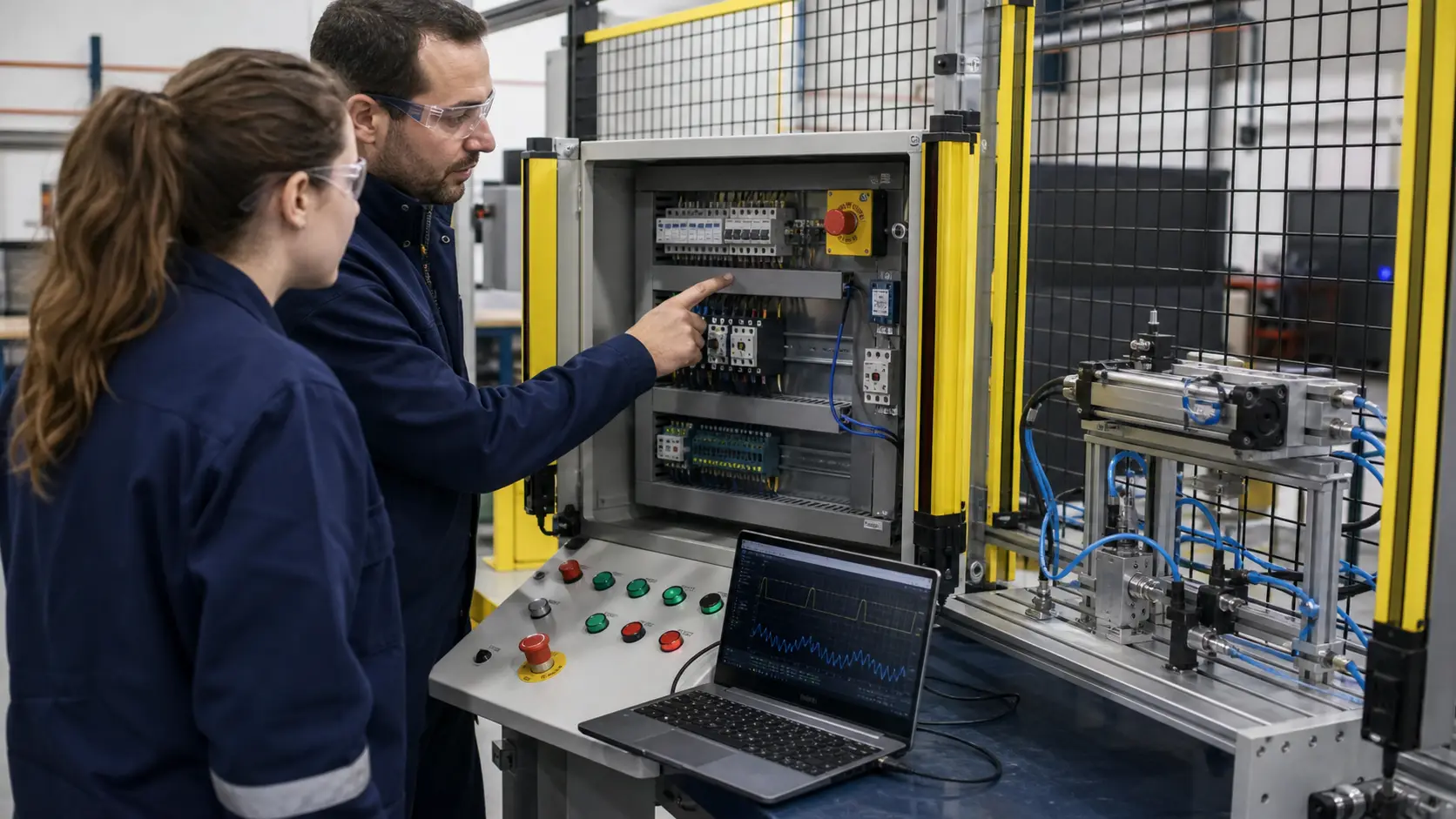
an instructor and maintenance learner tracing a guarded safety and actuator signal path in an isolated diagnostic cell while studying evidence-led PLC and machine fault isolation
The scene keeps evidence-led PLC and machine fault isolation connected to declared conditions, observable behavior, diagnostic boundaries and evidence that another person can reproduce.

System map / 02

Six concepts that control the result

Treat these as connected checkpoints. Each checkpoint has an expected state, an observable state and a boundary to the next part of the system. That structure prevents a software indication from being mistaken for physical proof.

NODE 01observable

Define the operating contract

safe state, precise symptom, operating mode, last known good condition, recent change, alarms, timestamps, drawings, access and acceptance criteria. For evidence-led PLC and machine fault isolation, record the initial condition, actor, requested change, observable result and stopping condition before selecting a tool or implementation.

NODE 02observable

Map the evidence path

physical condition through sensor, wiring, input, logic, output, interface, actuator, process response and independent feedback. Separate request, internal state, output or service, physical or user-visible result and independent feedback so each boundary can be inspected.

NODE 03observable

Prove normal operation

one normal command-response path measured and timed before introducing a controlled failure. Run more than one cycle from a known state and retain the values, timings or artifacts that demonstrate repeatability.

NODE 04observable

Exercise a boundary case

intermittent signal, stale network data, retained state, power return, mode conflict, sequence timeout and multiple symptoms. Choose minimum, maximum, simultaneous, delayed or restart conditions that reveal assumptions hidden by the happy path.

NODE 05observable

Diagnose a controlled fault

the first mechanical, electrical, I/O, program, communications, actuator, process or feedback disagreement. Preserve the first symptom, divide the system at a measurable boundary and change one condition only after predicting the result.

NODE 06observable

Transfer and hand over

cause removed, temporary changes cleared, regression cases passed and handover evidence retained. Restore normal state, remove temporary changes, repeat affected checks and document which claims remain limited to the learning environment.

Procedure / 03

A six-step practice and commissioning workflow

Run the steps in order the first time. Later, the same structure becomes a diagnostic loop: define the expected condition, observe the boundary, interpret the difference and choose one proving action.

  1. 01

    Write the acceptance case

    Convert safe state, precise symptom, operating mode, last known good condition, recent change, alarms, timestamps, drawings, access and acceptance criteria into initial conditions, one stimulus and observable pass criteria.

    Evidence: Another person can repeat the case without guessing the intended result.

    Avoid: Using page completion or an animation as the acceptance criterion.

  2. 02

    Build the map

    Document physical condition through sensor, wiring, input, logic, output, interface, actuator, process response and independent feedback and name who owns each state or decision.

    Evidence: Every request and result has a source, destination and useful inspection point.

    Avoid: Using the same value as command, status and independent feedback.

  3. 03

    Run the baseline

    Apply one normal command-response path measured and timed before introducing a controlled failure from a clean start and record the expected evidence.

    Evidence: Repeated runs produce the same bounded result.

    Avoid: Changing several parameters before a baseline exists.

  4. 04

    Challenge assumptions

    Test intermittent signal, stale network data, retained state, power return, mode conflict, sequence timeout and multiple symptoms without changing the acceptance contract.

    Evidence: Limits, timing and restart behavior reach defined states.

    Avoid: Testing only one ideal sequence.

  5. 05

    Isolate one failure

    Introduce or analyse the first mechanical, electrical, i/o, program, communications, actuator, process or feedback disagreement and locate the first disagreement.

    Evidence: The proving action distinguishes the leading hypotheses.

    Avoid: Resetting, forcing or replacing before evidence is retained.

  6. 06

    Close the evidence loop

    Complete cause removed, temporary changes cleared, regression cases passed and handover evidence retained and repeat the affected regression cases.

    Evidence: Reference use is complete when inputs, assumptions, units or initial conditions are recorded and the result is independently checked at a useful boundary.

    Avoid: Treating an acknowledged message or one successful rerun as handover.

Diagnostic matrix / 04

Symptoms, proving points and next actions

The table is a reasoning aid, not a parts-replacement chart. Preserve the initial symptom, inspect the named boundary and use the interpretation to choose the next controlled test. Site safety procedures and equipment manuals remain authoritative.

Diagnostic symptoms, inspection points, interpretations and next actions for PLC fault-finding guide: implementation, evidence and troubleshooting
Observed symptomInspectInterpretationNext proving action
The expected result is unclearRequirement, initial state, actor, stimulus, units and pass conditionThe technician, programmer and reviewer may be solving different versions of the task.Rewrite one observable acceptance case before continuing.
Internal state changes but the outcome does notRequest, final owner, output or service boundary and independent feedbackA software or interface indication proves intent at one layer, not the complete outcome.Trace the first boundary after the changing state.
Normal case passes but an edge case failsLimits, timing, simultaneous events, reset and restart assumptionsThe implementation contains a hidden assumption exposed by the changed condition.Add the failed boundary as a permanent regression case.
The failure disappears after resetOriginal symptom, histories, diagnostics, timestamps and active causeReset changed evidence or state without proving the initiating cause.Reproduce under a controlled condition and preserve pre/post-event data.
Simulator and target disagreeModel boundary, software version, task timing, I/O behavior, data types and configurationA learning model and the intended target do not share one of the recorded assumptions.Reduce the case and verify against current target documentation.
The result cannot be explainedPrediction, observation, proving action, alternative hypotheses and limitationsActivity occurred but the evidence is not yet transferable or reviewable.Have the learner defend the signal path and repeat a changed case.

Product evidence / 05

What the browser practice can actually demonstrate

The page connects definitions and worked examples to runnable tools, explicit assumptions and repeatable checks so a formula or pattern can be challenged.

Where simulation stops

The guide cannot authorize live electrical work or replace site energy control, drawings, risk assessment, qualified supervision and equipment manuals.

Commissioning notebook / 06

Six cases that turn the concepts into evidence

Use these as written briefs rather than click-through instructions. For every case, state the expected condition before acting, retain the first useful observation and explain why the final result proves the requirement. A different program or component choice can still be correct when it produces the same bounded behavior and evidence.

Case 01

predict → observe → prove

Prove define the operating contract

Engineering context. safe state, precise symptom, operating mode, last known good condition, recent change, alarms, timestamps, drawings, access and acceptance criteria. For evidence-led PLC and machine fault isolation, record the initial condition, actor, requested change, observable result and stopping condition before selecting a tool or implementation. Begin with a written normal condition and identify which request, state, physical result or communication value will provide independent confirmation. Do not begin by changing the configuration; the initial state is part of the evidence and should remain reproducible.

Controlled setup. Use the “Write the acceptance case” stage of the workflow: convert safe state, precise symptom, operating mode, last known good condition, recent change, alarms, timestamps, drawings, access and acceptance criteria into initial conditions, one stimulus and observable pass criteria. The acceptance record should show this result: another person can repeat the case without guessing the intended result. Record initial conditions, the exact stimulus and the observation point so another learner can repeat the case without relying on your memory.

Fault challenge. Introduce or analyse “The expected result is unclear” as one bounded deviation. Inspect requirement, initial state, actor, stimulus, units and pass condition The working interpretation is that the technician, programmer and reviewer may be solving different versions of the task. The next proving action is to rewrite one observable acceptance case before continuing. Change only one condition before observing the result, and preserve timestamps or measurements where timing matters.

Review and recovery. The most common trap here is using page completion or an animation as the acceptance criterion. After restoring the cause, repeat the normal case and at least one stop, timeout, disconnect or restart boundary relevant to this topic. Remove temporary forces and bypasses, return the model to a known state and retain the evidence that both operation and recovery are deliberate.

Explain it aloud: What is the fastest reliable PLC fault-finding method? A defensible short answer is: Define the symptom and expected state, preserve diagnostics, trace the signal path and use one measurement to split the remaining hypotheses at a useful boundary.

Case 02

predict → observe → prove

Prove map the evidence path

Engineering context. physical condition through sensor, wiring, input, logic, output, interface, actuator, process response and independent feedback. Separate request, internal state, output or service, physical or user-visible result and independent feedback so each boundary can be inspected. Begin with a written normal condition and identify which request, state, physical result or communication value will provide independent confirmation. Do not begin by changing the configuration; the initial state is part of the evidence and should remain reproducible.

Controlled setup. Use the “Build the map” stage of the workflow: document physical condition through sensor, wiring, input, logic, output, interface, actuator, process response and independent feedback and name who owns each state or decision. The acceptance record should show this result: every request and result has a source, destination and useful inspection point. Record initial conditions, the exact stimulus and the observation point so another learner can repeat the case without relying on your memory.

Fault challenge. Introduce or analyse “Internal state changes but the outcome does not” as one bounded deviation. Inspect request, final owner, output or service boundary and independent feedback The working interpretation is that a software or interface indication proves intent at one layer, not the complete outcome. The next proving action is to trace the first boundary after the changing state. Change only one condition before observing the result, and preserve timestamps or measurements where timing matters.

Review and recovery. The most common trap here is using the same value as command, status and independent feedback. After restoring the cause, repeat the normal case and at least one stop, timeout, disconnect or restart boundary relevant to this topic. Remove temporary forces and bypasses, return the model to a known state and retain the evidence that both operation and recovery are deliberate.

Explain it aloud: Why should I avoid resetting a PLC immediately? A defensible short answer is: A reset can remove active status, history or reproducible state. Preserve evidence first unless the approved safety response requires immediate action.

Case 03

predict → observe → prove

Prove prove normal operation

Engineering context. one normal command-response path measured and timed before introducing a controlled failure. Run more than one cycle from a known state and retain the values, timings or artifacts that demonstrate repeatability. Begin with a written normal condition and identify which request, state, physical result or communication value will provide independent confirmation. Do not begin by changing the configuration; the initial state is part of the evidence and should remain reproducible.

Controlled setup. Use the “Run the baseline” stage of the workflow: apply one normal command-response path measured and timed before introducing a controlled failure from a clean start and record the expected evidence. The acceptance record should show this result: repeated runs produce the same bounded result. Record initial conditions, the exact stimulus and the observation point so another learner can repeat the case without relying on your memory.

Fault challenge. Introduce or analyse “Normal case passes but an edge case fails” as one bounded deviation. Inspect limits, timing, simultaneous events, reset and restart assumptions The working interpretation is that the implementation contains a hidden assumption exposed by the changed condition. The next proving action is to add the failed boundary as a permanent regression case. Change only one condition before observing the result, and preserve timestamps or measurements where timing matters.

Review and recovery. The most common trap here is changing several parameters before a baseline exists. After restoring the cause, repeat the normal case and at least one stop, timeout, disconnect or restart boundary relevant to this topic. Remove temporary forces and bypasses, return the model to a known state and retain the evidence that both operation and recovery are deliberate.

Explain it aloud: What should I learn first about evidence-led PLC and machine fault isolation? A defensible short answer is: Start with the operating contract and evidence path: safe state, precise symptom, operating mode, last known good condition, recent change, alarms, timestamps, drawings, access and acceptance criteria, followed by physical condition through sensor, wiring, input, logic, output, interface, actuator, process response and independent feedback. Add advanced features only after the baseline is predictable.

Case 04

predict → observe → prove

Prove exercise a boundary case

Engineering context. intermittent signal, stale network data, retained state, power return, mode conflict, sequence timeout and multiple symptoms. Choose minimum, maximum, simultaneous, delayed or restart conditions that reveal assumptions hidden by the happy path. Begin with a written normal condition and identify which request, state, physical result or communication value will provide independent confirmation. Do not begin by changing the configuration; the initial state is part of the evidence and should remain reproducible.

Controlled setup. Use the “Challenge assumptions” stage of the workflow: test intermittent signal, stale network data, retained state, power return, mode conflict, sequence timeout and multiple symptoms without changing the acceptance contract. The acceptance record should show this result: limits, timing and restart behavior reach defined states. Record initial conditions, the exact stimulus and the observation point so another learner can repeat the case without relying on your memory.

Fault challenge. Introduce or analyse “The failure disappears after reset” as one bounded deviation. Inspect original symptom, histories, diagnostics, timestamps and active cause The working interpretation is that reset changed evidence or state without proving the initiating cause. The next proving action is to reproduce under a controlled condition and preserve pre/post-event data. Change only one condition before observing the result, and preserve timestamps or measurements where timing matters.

Review and recovery. The most common trap here is testing only one ideal sequence. After restoring the cause, repeat the normal case and at least one stop, timeout, disconnect or restart boundary relevant to this topic. Remove temporary forces and bypasses, return the model to a known state and retain the evidence that both operation and recovery are deliberate.

Explain it aloud: How do I practise evidence-led PLC and machine fault isolation effectively? A defensible short answer is: Use short cases with known initial conditions, a written prediction, one action and an observable result. Then alter a boundary or fault and explain why the evidence changed.

Case 05

predict → observe → prove

Prove diagnose a controlled fault

Engineering context. the first mechanical, electrical, I/O, program, communications, actuator, process or feedback disagreement. Preserve the first symptom, divide the system at a measurable boundary and change one condition only after predicting the result. Begin with a written normal condition and identify which request, state, physical result or communication value will provide independent confirmation. Do not begin by changing the configuration; the initial state is part of the evidence and should remain reproducible.

Controlled setup. Use the “Isolate one failure” stage of the workflow: introduce or analyse the first mechanical, electrical, i/o, program, communications, actuator, process or feedback disagreement and locate the first disagreement. The acceptance record should show this result: the proving action distinguishes the leading hypotheses. Record initial conditions, the exact stimulus and the observation point so another learner can repeat the case without relying on your memory.

Fault challenge. Introduce or analyse “Simulator and target disagree” as one bounded deviation. Inspect model boundary, software version, task timing, I/O behavior, data types and configuration The working interpretation is that a learning model and the intended target do not share one of the recorded assumptions. The next proving action is to reduce the case and verify against current target documentation. Change only one condition before observing the result, and preserve timestamps or measurements where timing matters.

Review and recovery. The most common trap here is resetting, forcing or replacing before evidence is retained. After restoring the cause, repeat the normal case and at least one stop, timeout, disconnect or restart boundary relevant to this topic. Remove temporary forces and bypasses, return the model to a known state and retain the evidence that both operation and recovery are deliberate.

Explain it aloud: What counts as proof of competence? A defensible short answer is: A repeatable artifact or system result plus an explanation of the signal path is stronger than time spent, screenshots or a copied answer. Physical competence requires separate supervised evidence.

Case 06

predict → observe → prove

Prove transfer and hand over

Engineering context. cause removed, temporary changes cleared, regression cases passed and handover evidence retained. Restore normal state, remove temporary changes, repeat affected checks and document which claims remain limited to the learning environment. Begin with a written normal condition and identify which request, state, physical result or communication value will provide independent confirmation. Do not begin by changing the configuration; the initial state is part of the evidence and should remain reproducible.

Controlled setup. Use the “Close the evidence loop” stage of the workflow: complete cause removed, temporary changes cleared, regression cases passed and handover evidence retained and repeat the affected regression cases. The acceptance record should show this result: reference use is complete when inputs, assumptions, units or initial conditions are recorded and the result is independently checked at a useful boundary. Record initial conditions, the exact stimulus and the observation point so another learner can repeat the case without relying on your memory.

Fault challenge. Introduce or analyse “The result cannot be explained” as one bounded deviation. Inspect prediction, observation, proving action, alternative hypotheses and limitations The working interpretation is that activity occurred but the evidence is not yet transferable or reviewable. The next proving action is to have the learner defend the signal path and repeat a changed case. Change only one condition before observing the result, and preserve timestamps or measurements where timing matters.

Review and recovery. The most common trap here is treating an acknowledged message or one successful rerun as handover. After restoring the cause, repeat the normal case and at least one stop, timeout, disconnect or restart boundary relevant to this topic. Remove temporary forces and bypasses, return the model to a known state and retain the evidence that both operation and recovery are deliberate.

Explain it aloud: Why test faults and restart behavior? A defensible short answer is: Because the first mechanical, electrical, i/o, program, communications, actuator, process or feedback disagreement or intermittent signal, stale network data, retained state, power return, mode conflict, sequence timeout and multiple symptoms can expose assumptions that never appear during ideal startup and steady operation.

Answer surface / 07

Questions people ask about PLC fault-finding guide

These concise answers define the operating, training and product boundaries most often missed in broad summaries. The full workflow and diagnostic table above provide the evidence behind them.

What is the fastest reliable PLC fault-finding method?

Define the symptom and expected state, preserve diagnostics, trace the signal path and use one measurement to split the remaining hypotheses at a useful boundary.

Why should I avoid resetting a PLC immediately?

A reset can remove active status, history or reproducible state. Preserve evidence first unless the approved safety response requires immediate action.

What should I learn first about evidence-led PLC and machine fault isolation?

Start with the operating contract and evidence path: safe state, precise symptom, operating mode, last known good condition, recent change, alarms, timestamps, drawings, access and acceptance criteria, followed by physical condition through sensor, wiring, input, logic, output, interface, actuator, process response and independent feedback. Add advanced features only after the baseline is predictable.

How do I practise evidence-led PLC and machine fault isolation effectively?

Use short cases with known initial conditions, a written prediction, one action and an observable result. Then alter a boundary or fault and explain why the evidence changed.

What counts as proof of competence?

A repeatable artifact or system result plus an explanation of the signal path is stronger than time spent, screenshots or a copied answer. Physical competence requires separate supervised evidence.

Why test faults and restart behavior?

Because the first mechanical, electrical, i/o, program, communications, actuator, process or feedback disagreement or intermittent signal, stale network data, retained state, power return, mode conflict, sequence timeout and multiple symptoms can expose assumptions that never appear during ideal startup and steady operation.

Can browser practice replace official software or hardware?

No. It can build concepts and diagnostic reasoning. Exact firmware, I/O electrical behavior, networking, safety and commissioning require current official tools, documentation and target equipment.

How should progress be documented?

Keep the requirement, initial state, program or configuration, observed values, fault hypothesis, proving action, recovery result and a concise limitations statement.