PID Control for PLCs: Practical Tuning Guide

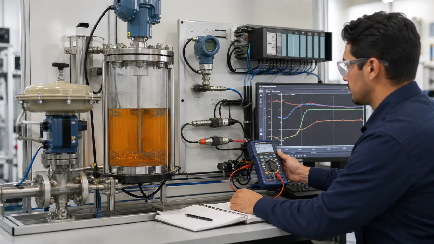
If your process — temperature, pressure, level, flow — drifts away from setpoint and you need it to stay put, a PID controller is almost certainly the right tool. And in industrial automation, that PID runs inside a PLC.

A PID (Proportional-Integral-Derivative) controller continuously computes an output signal that drives a process variable toward a setpoint by correcting for current error (P), accumulated past error (I), and predicted future error (D). Understanding each term lets you tune a controller without guesswork.

The Control Loop

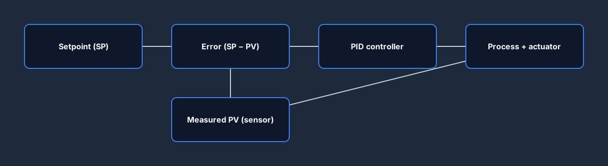
Before PID makes sense, the closed-loop control structure must be clear:

1. Setpoint (SP) — the target value you want the process at (e.g., 75°C).
2. Process Variable (PV) — the measured value from the sensor (e.g., actual temperature).
3. Error (e) — the difference: e = SP - PV.
4. PID output (CV / Manipulated Variable) — the signal sent to the actuator (e.g., 0–100% heater power, valve position).

The PLC reads the sensor, computes the PID output, writes it to the actuator, and repeats every sample interval. This is the closed feedback loop the rest of the guide builds on: the measured PV is subtracted from the setpoint to form the error that the PID controller acts on.

The Three Terms

Proportional (P)

P_Output := Kp * Error;

The proportional term produces an output directly proportional to the current error. Large error → large output. If the process is 10°C below setpoint and Kp = 2.0, the P contribution is 20 (in whatever output units).

Effect of Kp:

• Too low: sluggish response, large steady-state offset.
• Too high: oscillation, potentially instability.

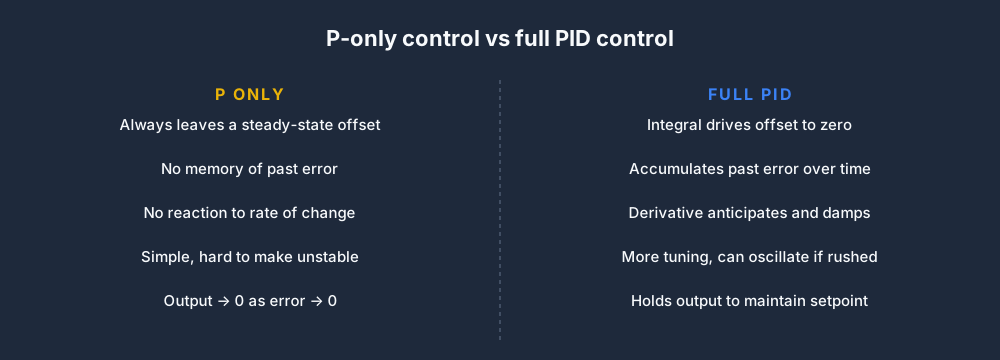
Proportional control alone always has a residual steady-state error (also called offset) because when error → 0, output → 0, but some output is always needed to maintain setpoint against losses.

Integral (I)

Integral := Integral + (Error * SampleTime);
I_Output := Ki * Integral;

The integral term accumulates error over time. If the process sits below setpoint for a long time, the integral builds up and pushes the output higher until the process variable reaches setpoint. This eliminates steady-state offset.

Effect of Ki:

• Too low: slow elimination of offset.
• Too high: overshoot, slow oscillation (integral windup).

Integral windup occurs when the output saturates (hits 0% or 100%) but the integral keeps accumulating because the process never reaches setpoint. On output unsaturation, the accumulated integral causes a large overshoot. Anti-windup clamps the integral when the output is saturated.

Derivative (D)

D_Output := Kd * (Error - PrevError) / SampleTime;
PrevError := Error;

The derivative term predicts where the error is heading based on its rate of change. If error is decreasing rapidly, D reduces the output to prevent overshoot. If error is increasing rapidly, D increases the output for a faster response.

Effect of Kd:

• Too low: overshoot on fast disturbances.
• Too high: amplifies noise, causes chatter in the output.

Derivative action is often applied to the process variable rather than the error (Kd * (PrevPV - PV) / SampleTime) to avoid a "derivative kick" when the setpoint changes abruptly.

What Each Term Fixes

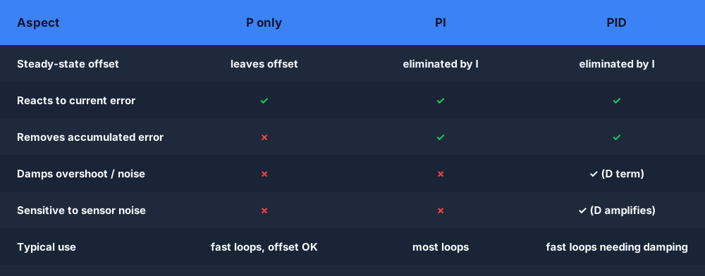
Put the three terms side by side and the role of each becomes clear: P alone leaves an offset, I removes it, and D damps the overshoot the first two can introduce.

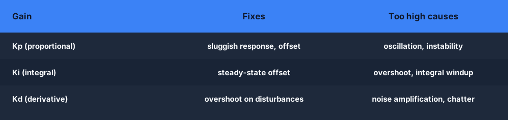
The other way to read the same trade-offs is by what happens when you push each gain too far.

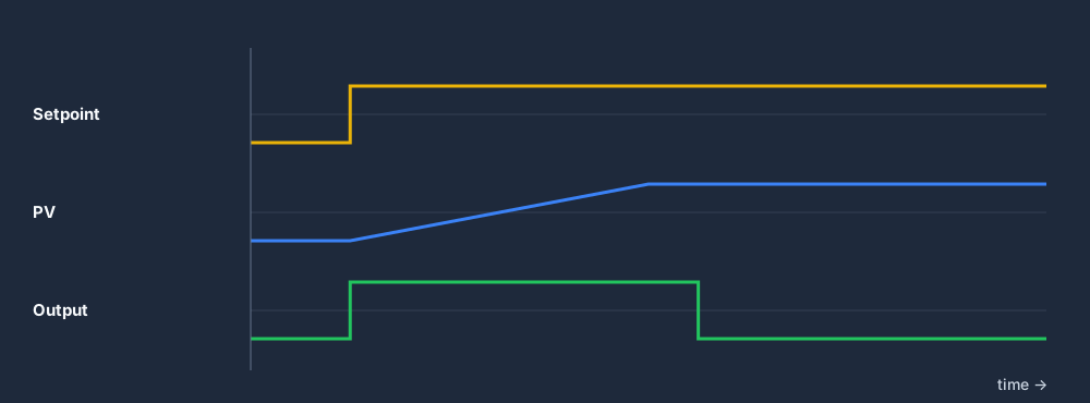
A well-tuned loop responds to a setpoint step by rising and settling cleanly on target, with the controller output backing off as the process variable arrives (the curve below is illustrative, not measured data).

Complete PID Algorithm in IEC 61131-3

(* Positional PID with anti-windup and output clamping *)
(* Call this block every SampleTime seconds in a periodic task *)

Error    := Setpoint - ProcessVar;
Integral := Integral + (Error * SampleTime);

(* Anti-windup: clamp integral contribution *)
IF Output >= OutputMax THEN
    Integral := Integral - (Error * SampleTime);  (* Unwind *)
END_IF;
IF Output <= OutputMin THEN
    Integral := Integral - (Error * SampleTime);
END_IF;

Derivative := (Error - PrevError) / SampleTime;

Output := (Kp * Error) + (Ki * Integral) + (Kd * Derivative);
Output := MAX(OutputMin, MIN(OutputMax, Output));  (* Clamp *)

PrevError := Error;

Variable declarations:

VAR
    Error, PrevError : REAL := 0.0;
    Integral         : REAL := 0.0;
    Derivative       : REAL := 0.0;
    Output           : REAL := 0.0;
    Kp, Ki, Kd       : REAL;          (* Tuning parameters *)
    Setpoint         : REAL;
    ProcessVar       : REAL;
    SampleTime       : REAL := 0.1;   (* 100 ms default *)
    OutputMin        : REAL := 0.0;
    OutputMax        : REAL := 100.0;
END_VAR;

Consistent Sample Time is Critical

The PID algorithm assumes it is called at a consistent SampleTime interval. If the call interval varies, the integral and derivative calculations are wrong.

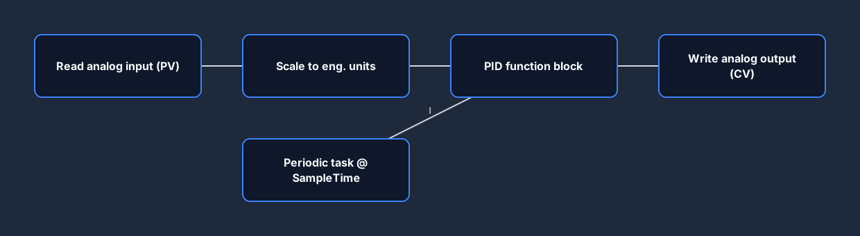
Solution: put the PID function block in a periodic task configured for the sample period (e.g., 100 ms). Do not put it in the main cyclic task where scan time can vary. IEC 61131-3 platforms and modern PLCs support task configuration for this purpose.

Inside that periodic task the order of operations is fixed: read the analog input, scale it to engineering units, run the PID block, then write the analog output — every sample interval.

Practical Tuning Methods

Manual Tuning (Start Here for Simple Loops)

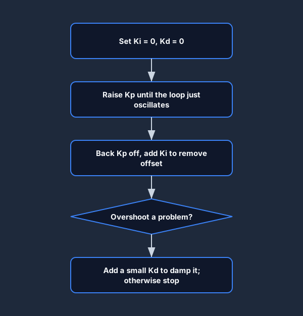
The whole procedure follows one simple order — get P right, add I to kill the offset, then add D only if you need it.

1. Set Ki = 0, Kd = 0. Increase Kp until the process oscillates. The Kp at which oscillation begins is the ultimate gain Ku.
2. Record the period of oscillation Tu.
3. Start with Kp = 0.45 * Ku and Ki = 0.54 * Ku / Tu. This is a conservative first guess.
4. Add Kd only if overshoot is a problem. Start small: Kd = 0.05 * Kp * Tu.
5. Fine-tune by observation: if there is still steady-state offset, increase Ki. If there is overshoot, reduce Ki or add Kd.

Auto-Tune

Many PLC PID function blocks include an auto-tune feature that applies a step change to the output, observes the process response, and computes initial PID gains. Auto-tune gives a usable starting point, not a final set of parameters — expect to refine by observation.

Ziegler-Nichols Step Response Method

For a process with known gain and time constant (from a step test), the Ziegler-Nichols step response method provides an initial tuning formula. It tends to give aggressive settings — good for quick response but often with overshoot. Start with half the calculated Ki for more conservative control.

Tuning Tips That Save Hours

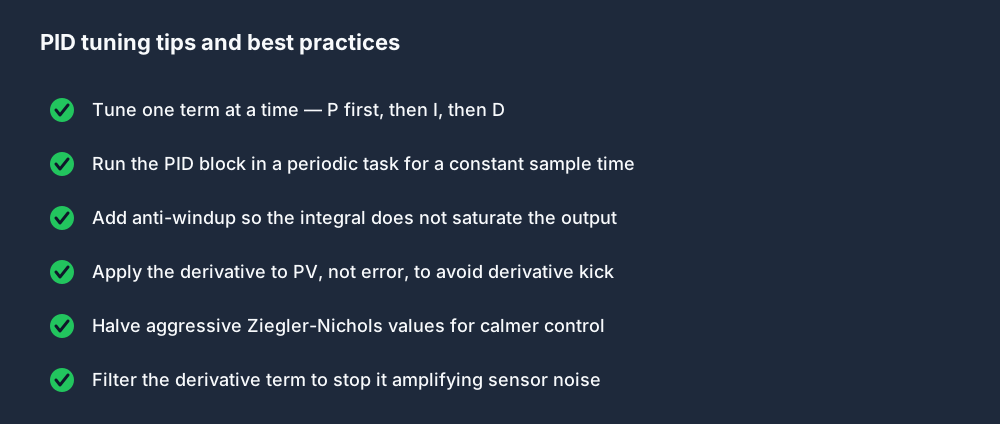
Whichever method you start from, a handful of habits keep a loop stable and easy to commission.

Why Not Just Use P?

It is tempting to skip the integral and derivative terms, but a proportional-only controller can never sit exactly on setpoint. Seeing P-only and full PID side by side makes the case for the extra two terms.

PID in Allen-Bradley and Siemens

Allen-Bradley

AB provides the PID instruction as part of Studio 5000. Key parameters:

• SP (setpoint), PV (process variable), CV (control variable / output).
• Kp, Ki (integral in repeats/min), Kd (derivative in minutes).
• Note: AB typically expresses Ki in "repeats per minute" rather than a direct gain — convert if comparing with IEC PID implementations.

Siemens TIA Portal

TIA Portal provides PID_Compact and PID_3Step function blocks. PID_Compact is the standard continuous output PID. It includes auto-tune (pre-tuning and fine tuning modes) and integrates with the TIA Portal commissioning panel for graphical tuning.

Real-World PID Scenarios in the Simulator

The PID Temperature Control (pid-temp) scenario lets you tune a heating loop: write the PID rung, set Kp, Ki, Kd, and watch the simulated temperature trend settle on setpoint. The auto-grader checks that:

• Setpoint is reached within the time limit.
• Steady-state error is within ±2°C.
• Output does not oscillate after settling.

Before writing any PID rung, it helps to understand where the loop lives on the process drawing — reading the P&ID for this loop shows you which tag is the transmitter, which is the controller, and which drives the valve.

For analogue signal handling and engineering unit scaling, read the Analog IO and Scaling lesson.

---

Practice this yourself in the simulator — 3 scenarios free. No install. No credit card. Write real ladder logic against a live machine model in your browser.

Try the simulator free →