PLC Simulator
PLC field notesinstrumentation

Pressure Transmitter Working Principle: 4–20 mA

Trace pressure through the diaphragm, sensing bridge and electronics into a 4–20 mA PLC input, with scaling, wiring and fault examples.

PLC Simulation Software13 min read

Direct answer: Process pressure deflects a metal diaphragm by a tiny amount. A sensing element—often piezoresistive, capacitive or strain-gauge based—converts that deformation into an electrical change. Transmitter electronics compensate, linearise and scale it into a robust signal such as 4–20 mA for a PLC analog input.
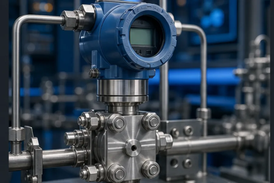
Industrial pressure transmitter mounted on a process training skid

The useful causal chain is pressure → force on area → diaphragm deflection → electrical change → conditioned signal → engineering value. Understanding it explains why a blocked impulse line, damaged diaphragm and open current loop produce different symptoms.

Stage 1: pressure reaches the diaphragm
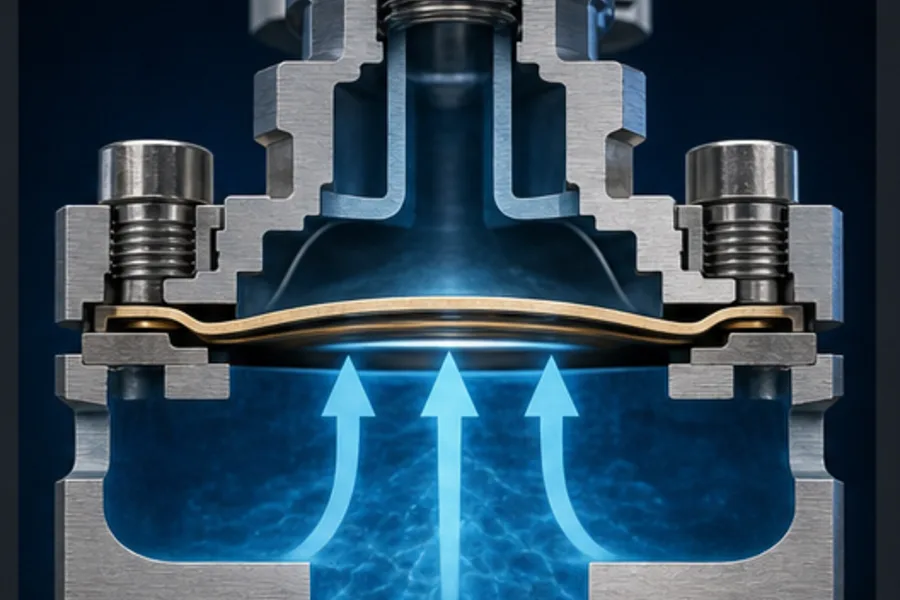
Cutaway showing process pressure deflecting a transmitter isolation diaphragm

The process connection exposes a wetted diaphragm or transmits pressure through fill fluid to an internal sensing diaphragm. Pressure is force per unit area, so the diaphragm deflects predictably within its elastic range.

The movement is extremely small. A transmitter is not a pressure switch with a large mechanical snap. It continuously measures deformation across a range.

Diaphragm material, process seal, fill fluid and connection must match pressure, temperature, corrosion, hygiene and overpressure requirements. A chemically incompatible but electrically correct transmitter is still a wrong selection.

Stage 2: deformation becomes an electrical signal
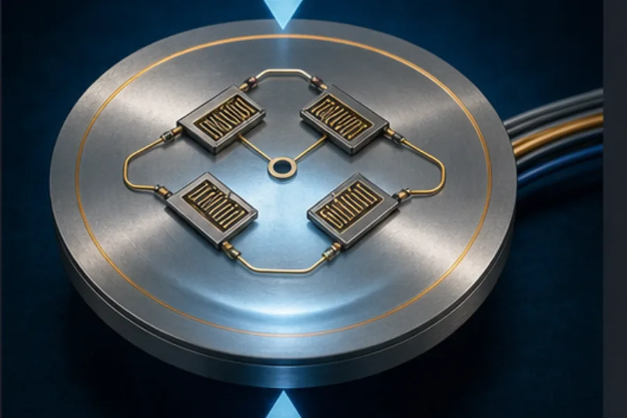
Strain-gauge sensing bridge responding to tiny pressure-diaphragm movement

Common sensing methods include:

  • Piezoresistive/strain gauge: resistance changes as the element stretches or compresses, commonly arranged as a bridge.
  • Capacitive: diaphragm movement changes the spacing/capacitance between electrodes.
  • Resonant or other specialised methods: pressure changes a measured physical property suited to high accuracy or demanding service.

In a Wheatstone-bridge style sensor, tiny resistance changes create a differential voltage. Temperature also affects materials, so the electronics apply compensation based on calibration data.

Stage 3: electronics linearise and scale
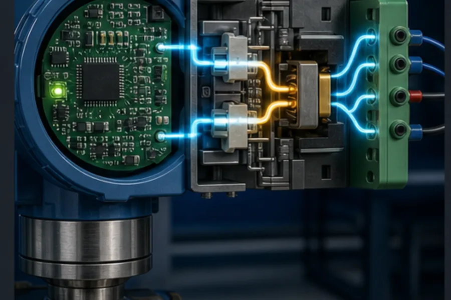
Pressure transmitter electronics conditioning a sensor bridge into a current-loop signal

The electronics amplify the small sensor signal, correct non-linearity and temperature effects, apply range/zero calibration, and drive the output. Smart transmitters may add HART or another protocol over/alongside the analog signal.

Important terms:

Reference tableSwipe
TermMeaning
LRVlower range value; process value represented by 4 mA
URVupper range value; process value represented by 20 mA
SpanURV − LRV
Zeroconfigured lower endpoint, not always zero pressure
Turndownratio between sensor capability and configured span; excessive turndown can affect performance

A 0–10 bar transmitter ranged 0–10 bar maps 0 bar to 4 mA and 10 bar to 20 mA. A differential-pressure transmitter could instead map −100 to +100 mbar; 4 mA then represents −100 mbar, not physical zero.

Why industry uses 4–20 mA

Unlike a 0–20 mA loop, 4 mA is a live zero. A valid minimum measurement still carries current, while a broken wire can fall near 0 mA. Current is also comparatively robust over long cable runs because the receiver measures loop current rather than relying solely on a remote voltage level.

Linear scaling is:

Engineering value = LRV + (mA − 4) × (URV − LRV) / 16

For 0–10 bar:

  • 4 mA = 0 bar
  • 8 mA = 2.5 bar
  • 12 mA = 5 bar
  • 16 mA = 7.5 bar
  • 20 mA = 10 bar

Signals outside the normal range may represent underrange/overrange or a configured fault indication. Follow the transmitter and PLC module conventions; do not hardcode one universal threshold.

Two-wire loop to a PLC analog input
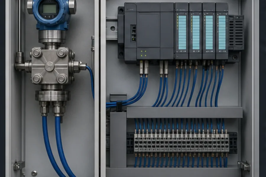
Two-wire pressure transmitter connected to a PLC analog input and power supply

A common two-wire transmitter uses the same loop for power and signal:

+24 V supply → transmitter +
transmitter − → PLC analog input +
PLC analog input −/return → 0 V supply

The exact path depends on whether the analog input is active/passive, isolated/shared and how the common is referenced. A loop calibrator can source or simulate current, but must be configured correctly to avoid putting two power sources into the same loop.

Check the loop's voltage budget: supply voltage must cover transmitter minimum voltage, input burden, barriers/isolators, cable drop and any other series device at 20 mA.

Shielding and earth practice follow the system design. Connecting a shield at arbitrary multiple points can create unwanted currents; leaving it floating against the drawing can reduce noise protection.

Gauge, absolute and differential pressure

  • Gauge pressure: referenced to local atmosphere. A tyre gauge is a familiar example.
  • Absolute pressure: referenced to an internal vacuum reference.
  • Differential pressure: measures the difference between two process connections.

Differential pressure transmitters can infer flow across a primary element, level from hydrostatic head, or filter condition from pressure drop. The transmitter measures differential pressure; PLC/configuration turns that into the desired process variable.

PLC scaling and diagnostics

The analog module converts current to raw counts. Scale those counts from the module's configured raw range—not a copied constant from another brand.

A robust analog-input function should produce:

  • raw input;
  • scaled engineering value and units;
  • underrange/overrange quality;
  • wire-break/bad-channel state;
  • filtered value if process dynamics justify it; and
  • simulation/maintenance state that is clearly visible.

Alarm logic should use engineering units and appropriate hysteresis/delay. Filtering a noisy signal too aggressively can hide a real fast process change.

What common failures look like

Reference tableSwipe
SymptomLikely zones
Near 0 mAopen loop, lost supply, failed transmitter
Fixed 4 mAtrue LRV, blocked impulse path, frozen configuration/simulation
Fixed high valueoverpressure, plugged low side on DP, wiring/configuration issue
Noisy readingprocess pulsation, grounding/shielding, loose connection, cavitation
Slow responseimpulse-line restriction, damping setting, viscous fill/process
Offsetzero shift, mounting/head effect, temperature, diaphragm damage

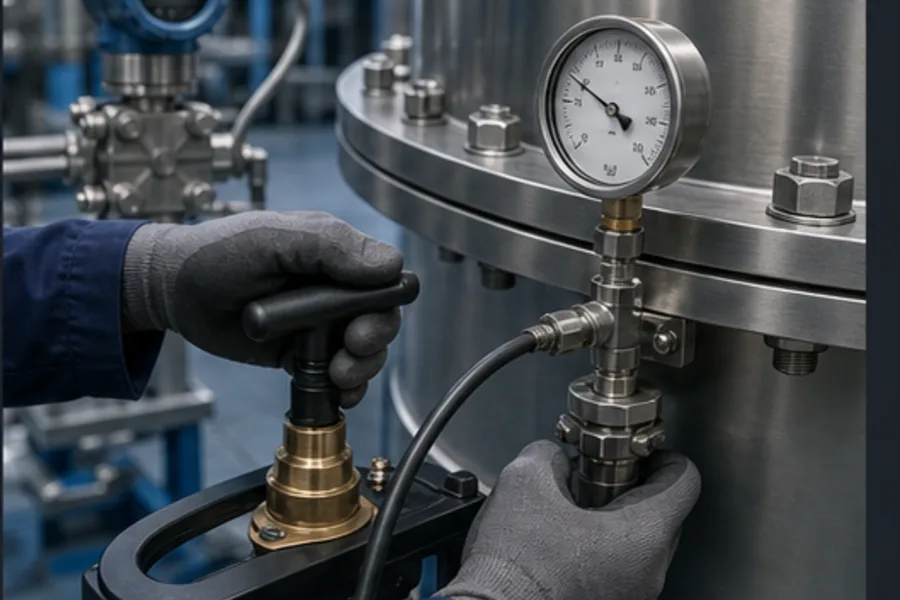
Pressure calibration check using a hand pump and reference gauge

Calibration compares applied reference pressure to transmitter output at controlled points. It is different from ranging, which changes LRV/URV, and from trimming, which adjusts sensor/output calibration. Record as-found and as-left data under the site's instrument procedure.

Safety and process isolation

Pressure systems can release hazardous fluid or stored energy. Isolate, depressurise, drain/vent and verify according to the approved process before opening impulse lines or removing a transmitter. Chemical compatibility, temperature and hazardous-area requirements are part of the instrument design.

Learn the mechanism and the PLC value together

Use the Pressure Transmitter lesson to change process pressure, watch the sensing story and inspect the PLC signal. The contextual Pro tutor can explain the specific sensor and current scenario without leaving the lesson.

Then practise engineering-unit handling in the analog input examples and 4–20 mA scaling calculator.

Frequently asked questions

What does a pressure transmitter do in one sentence?

It converts physical fluid/gas pressure into a standardized electrical value that a PLC, DCS or indicator can read.

Why does 4 mA represent zero?

It creates a live zero: the minimum valid measurement still proves loop current exists, while an open circuit can fall below the valid measurement range.

What is the difference between a pressure switch and transmitter?

A switch changes a discrete contact around a setpoint. A transmitter continuously reports pressure across a range, usually as 4–20 mA or digital data.

Can a pressure transmitter measure tank level?

Yes. In a known-density liquid, hydrostatic pressure corresponds to liquid head. Mounting elevation, density, vessel pressure and DP reference arrangement must be handled correctly.

Why can the PLC show pressure when the process is isolated?

Pressure may remain trapped, an impulse line may hold a hydraulic head, the input may be simulated, or the transmitter/scale may be offset. Verify the entire measurement chain safely.
Primary technical references

ShareX / TwitterLinkedIn

From reading to running logic

Turn pressure into a live PLC value

Change the process pressure and follow diaphragm movement through signal conditioning and analog scaling.

Open the pressure lesson

Continue learning

Related field notes

All articles
pneumatics
solenoid valve

How a Solenoid Valve Works: Coil to Flow

See how direct and pilot solenoid valves move a plunger or spool, how NO/NC states work, and how a PLC output controls the coil.

12 min read
automation
plc

Industrial Automation Components Map

Understand PLCs, I/O, sensors, relays, drives, valves, safety and HMIs as one closed control loop—with interactive component labs.

15 min read
electrical
contactor

Contactor Wiring Diagram: Power & PLC

Wire a contactor correctly: L1/L2/L3, T1/T2/T3, A1/A2, seal-in and PLC feedback explained with diagrams and an interactive cutaway.

13 min read

Technical reference and worked-example guide

Pressure transmitter working principle: implementation, evidence and troubleshooting

Direct answer

Pressure transmitter working principle becomes useful when it connects measurand, pressure reference, range, overpressure, process connection, wetted materials, sensing element, output, loop supply, input, scaling and accuracy with process pressure through mechanical sensing and electronic conversion to loop current, input counts, engineering units, display and control action, then proves zero, midrange and span points compared with a reference and expected current plus plc value under normal, boundary, fault and recovery conditions. The objective is a repeatable engineering or learning result, not merely activity inside a page or tool.

This guide is written for instrumentation and PLC learners tracing applied pressure through sensing element, electronics, current loop, analog input, scaling and control use. The intended result is specific: the reader can distinguish gauge, absolute and differential measurement, calculate loop values and diagnose zero, span, wiring, supply and impulse-line errors.

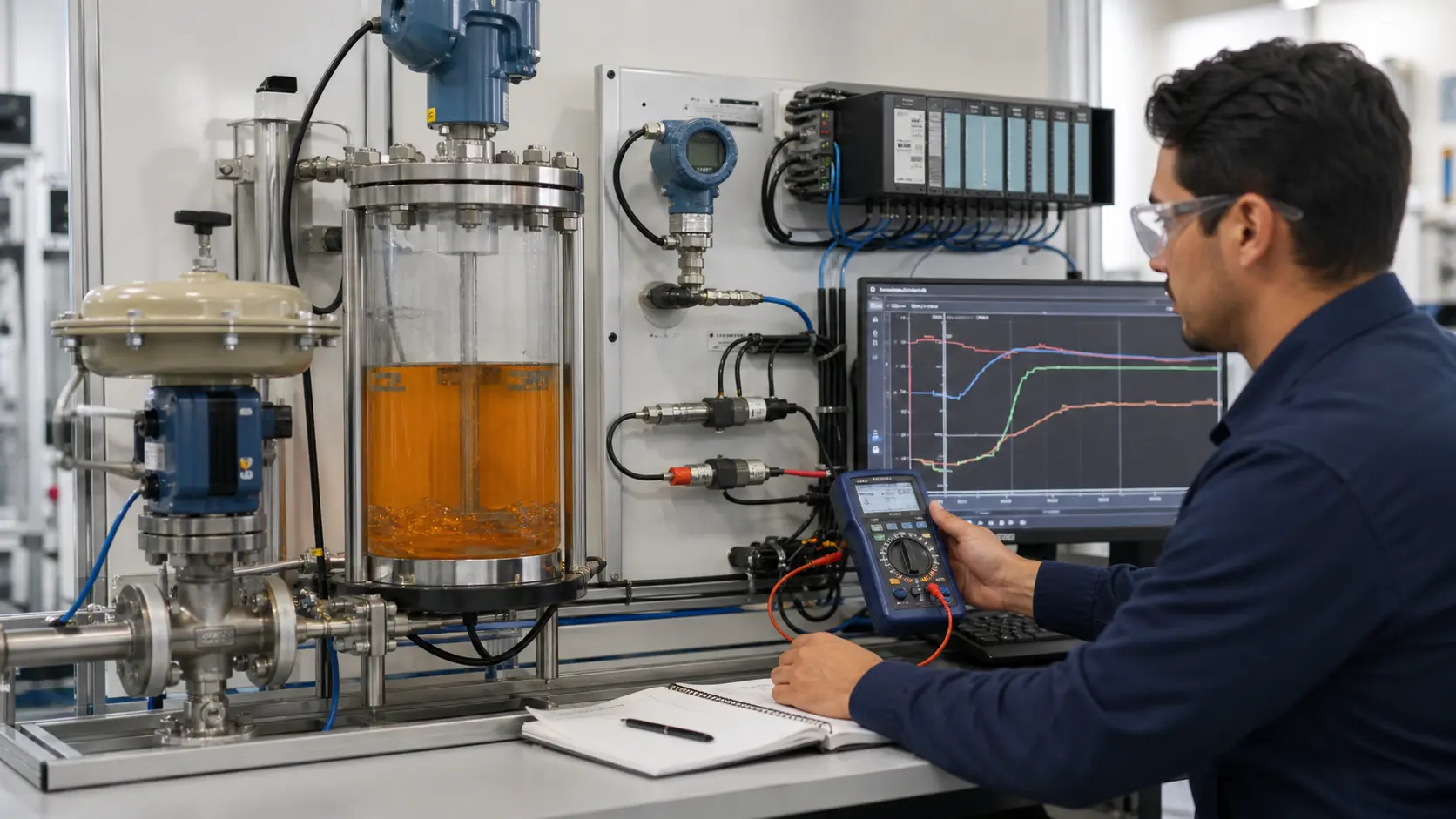
an instrumentation engineer correlating a process skid, transmitter, calibrator, PLC trend and actuator response while studying pressure sensing, 4–20 mA transmission and PLC interpretation
The physical context keeps pressure sensing, 4–20 mA transmission and PLC interpretation tied to declared inputs, owned decisions, observable results and evidence that another person can verify.

System map / 02

Six concepts that control the result

Treat these as connected checkpoints. Each checkpoint has an expected state, an observable state and a boundary to the next part of the system. That structure prevents a software indication from being mistaken for physical proof.

NODE 01observable

Define the operating contract

measurand, pressure reference, range, overpressure, process connection, wetted materials, sensing element, output, loop supply, input, scaling and accuracy. For pressure sensing, 4–20 mA transmission and PLC interpretation, record the initial condition, actor, requested change, observable result and stopping condition before selecting a tool or implementation.

NODE 02observable

Map the evidence path

process pressure through mechanical sensing and electronic conversion to loop current, input counts, engineering units, display and control action. Separate request, internal state, output or service, physical or user-visible result and independent feedback so each boundary can be inspected.

NODE 03observable

Prove normal operation

zero, midrange and span points compared with a reference and expected current plus PLC value. Run more than one cycle from a known state and retain the values, timings or artifacts that demonstrate repeatability.

NODE 04observable

Exercise a boundary case

plugged impulse line, trapped gas or liquid, leak, zero shift, overrange, insufficient loop voltage, open circuit, ground loop and scaling. Choose minimum, maximum, simultaneous, delayed or restart conditions that reveal assumptions hidden by the happy path.

NODE 05observable

Diagnose a controlled fault

a process, connection, sensing-element, transmitter, loop-power, wiring, input, scaling or display defect. Preserve the first symptom, divide the system at a measurable boundary and change one condition only after predicting the result.

NODE 06observable

Transfer and hand over

the loop verified with current data sheets, approved isolation and a traceable calibration procedure. Restore normal state, remove temporary changes, repeat affected checks and document which claims remain limited to the learning environment.

Procedure / 03

A six-step practice and commissioning workflow

Run the steps in order the first time. Later, the same structure becomes a diagnostic loop: define the expected condition, observe the boundary, interpret the difference and choose one proving action.

  1. 01

    Write the acceptance case

    Convert measurand, pressure reference, range, overpressure, process connection, wetted materials, sensing element, output, loop supply, input, scaling and accuracy into initial conditions, one stimulus and observable pass criteria.

    Evidence: Another person can repeat the case without guessing the intended result.

    Avoid: Using page completion or an animation as the acceptance criterion.

  2. 02

    Build the map

    Document process pressure through mechanical sensing and electronic conversion to loop current, input counts, engineering units, display and control action and name who owns each state or decision.

    Evidence: Every request and result has a source, destination and useful inspection point.

    Avoid: Using the same value as command, status and independent feedback.

  3. 03

    Run the baseline

    Apply zero, midrange and span points compared with a reference and expected current plus plc value from a clean start and record the expected evidence.

    Evidence: Repeated runs produce the same bounded result.

    Avoid: Changing several parameters before a baseline exists.

  4. 04

    Challenge assumptions

    Test plugged impulse line, trapped gas or liquid, leak, zero shift, overrange, insufficient loop voltage, open circuit, ground loop and scaling without changing the acceptance contract.

    Evidence: Limits, timing and restart behavior reach defined states.

    Avoid: Testing only one ideal sequence.

  5. 05

    Isolate one failure

    Introduce or analyse a process, connection, sensing-element, transmitter, loop-power, wiring, input, scaling or display defect and locate the first disagreement.

    Evidence: The proving action distinguishes the leading hypotheses.

    Avoid: Resetting, forcing or replacing before evidence is retained.

  6. 06

    Close the evidence loop

    Complete the loop verified with current data sheets, approved isolation and a traceable calibration procedure and repeat the affected regression cases.

    Evidence: Reference use is complete when inputs, assumptions, units or initial conditions are recorded and the result is independently checked at a useful boundary.

    Avoid: Treating an acknowledged message or one successful rerun as handover.

Diagnostic matrix / 04

Symptoms, proving points and next actions

The table is a reasoning aid, not a parts-replacement chart. Preserve the initial symptom, inspect the named boundary and use the interpretation to choose the next controlled test. Site safety procedures and equipment manuals remain authoritative.

Diagnostic symptoms, inspection points, interpretations and next actions for Pressure transmitter working principle: implementation, evidence and troubleshooting
Observed symptomInspectInterpretationNext proving action
The expected result is unclearRequirement, initial state, actor, stimulus, units and pass conditionThe technician, programmer and reviewer may be solving different versions of the task.Rewrite one observable acceptance case before continuing.
Internal state changes but the outcome does notRequest, final owner, output or service boundary and independent feedbackA software or interface indication proves intent at one layer, not the complete outcome.Trace the first boundary after the changing state.
Normal case passes but an edge case failsLimits, timing, simultaneous events, reset and restart assumptionsThe implementation contains a hidden assumption exposed by the changed condition.Add the failed boundary as a permanent regression case.
The failure disappears after resetOriginal symptom, histories, diagnostics, timestamps and active causeReset changed evidence or state without proving the initiating cause.Reproduce under a controlled condition and preserve pre/post-event data.
Simulator and target disagreeModel boundary, software version, task timing, I/O behavior, data types and configurationA learning model and the intended target do not share one of the recorded assumptions.Reduce the case and verify against current target documentation.
The result cannot be explainedPrediction, observation, proving action, alternative hypotheses and limitationsActivity occurred but the evidence is not yet transferable or reviewable.Have the learner defend the signal path and repeat a changed case.

Product evidence / 05

What the browser practice can actually demonstrate

The page connects definitions and worked examples to runnable tools, explicit assumptions and repeatable checks so a formula or pattern can be challenged.

Where simulation stops

The guide does not select pressure ratings, wetted materials, hazardous-area protection, manifolds or calibration intervals for a real process.

Commissioning notebook / 06

Six cases that turn the concepts into evidence

Use these as written briefs rather than click-through instructions. For every case, state the expected condition before acting, retain the first useful observation and explain why the final result proves the requirement. A different program or component choice can still be correct when it produces the same bounded behavior and evidence.

Case 01

predict → observe → prove

Prove define the operating contract

Engineering context. measurand, pressure reference, range, overpressure, process connection, wetted materials, sensing element, output, loop supply, input, scaling and accuracy. For pressure sensing, 4–20 mA transmission and PLC interpretation, record the initial condition, actor, requested change, observable result and stopping condition before selecting a tool or implementation. Begin with a written normal condition and identify which request, state, physical result or communication value will provide independent confirmation. Do not begin by changing the configuration; the initial state is part of the evidence and should remain reproducible.

Controlled setup. Use the “Write the acceptance case” stage of the workflow: convert measurand, pressure reference, range, overpressure, process connection, wetted materials, sensing element, output, loop supply, input, scaling and accuracy into initial conditions, one stimulus and observable pass criteria. The acceptance record should show this result: another person can repeat the case without guessing the intended result. Record initial conditions, the exact stimulus and the observation point so another learner can repeat the case without relying on your memory.

Fault challenge. Introduce or analyse “The expected result is unclear” as one bounded deviation. Inspect requirement, initial state, actor, stimulus, units and pass condition The working interpretation is that the technician, programmer and reviewer may be solving different versions of the task. The next proving action is to rewrite one observable acceptance case before continuing. Change only one condition before observing the result, and preserve timestamps or measurements where timing matters.

Review and recovery. The most common trap here is using page completion or an animation as the acceptance criterion. After restoring the cause, repeat the normal case and at least one stop, timeout, disconnect or restart boundary relevant to this topic. Remove temporary forces and bypasses, return the model to a known state and retain the evidence that both operation and recovery are deliberate.

Explain it aloud: How does a pressure transmitter work? A defensible short answer is: It converts deformation of a sensing element into an electrical signal, conditions and linearizes that signal, then transmits a standard output such as 4–20 mA.

Case 02

predict → observe → prove

Prove map the evidence path

Engineering context. process pressure through mechanical sensing and electronic conversion to loop current, input counts, engineering units, display and control action. Separate request, internal state, output or service, physical or user-visible result and independent feedback so each boundary can be inspected. Begin with a written normal condition and identify which request, state, physical result or communication value will provide independent confirmation. Do not begin by changing the configuration; the initial state is part of the evidence and should remain reproducible.

Controlled setup. Use the “Build the map” stage of the workflow: document process pressure through mechanical sensing and electronic conversion to loop current, input counts, engineering units, display and control action and name who owns each state or decision. The acceptance record should show this result: every request and result has a source, destination and useful inspection point. Record initial conditions, the exact stimulus and the observation point so another learner can repeat the case without relying on your memory.

Fault challenge. Introduce or analyse “Internal state changes but the outcome does not” as one bounded deviation. Inspect request, final owner, output or service boundary and independent feedback The working interpretation is that a software or interface indication proves intent at one layer, not the complete outcome. The next proving action is to trace the first boundary after the changing state. Change only one condition before observing the result, and preserve timestamps or measurements where timing matters.

Review and recovery. The most common trap here is using the same value as command, status and independent feedback. After restoring the cause, repeat the normal case and at least one stop, timeout, disconnect or restart boundary relevant to this topic. Remove temporary forces and bypasses, return the model to a known state and retain the evidence that both operation and recovery are deliberate.

Explain it aloud: How do you scale a 4–20 mA pressure transmitter in a PLC? A defensible short answer is: Map the input value corresponding to 4 mA to the lower range and 20 mA to the upper range, then test under-range, over-range and fault behavior.

Case 03

predict → observe → prove

Prove prove normal operation

Engineering context. zero, midrange and span points compared with a reference and expected current plus PLC value. Run more than one cycle from a known state and retain the values, timings or artifacts that demonstrate repeatability. Begin with a written normal condition and identify which request, state, physical result or communication value will provide independent confirmation. Do not begin by changing the configuration; the initial state is part of the evidence and should remain reproducible.

Controlled setup. Use the “Run the baseline” stage of the workflow: apply zero, midrange and span points compared with a reference and expected current plus plc value from a clean start and record the expected evidence. The acceptance record should show this result: repeated runs produce the same bounded result. Record initial conditions, the exact stimulus and the observation point so another learner can repeat the case without relying on your memory.

Fault challenge. Introduce or analyse “Normal case passes but an edge case fails” as one bounded deviation. Inspect limits, timing, simultaneous events, reset and restart assumptions The working interpretation is that the implementation contains a hidden assumption exposed by the changed condition. The next proving action is to add the failed boundary as a permanent regression case. Change only one condition before observing the result, and preserve timestamps or measurements where timing matters.

Review and recovery. The most common trap here is changing several parameters before a baseline exists. After restoring the cause, repeat the normal case and at least one stop, timeout, disconnect or restart boundary relevant to this topic. Remove temporary forces and bypasses, return the model to a known state and retain the evidence that both operation and recovery are deliberate.

Explain it aloud: What should I learn first about pressure sensing, 4–20 mA transmission and PLC interpretation? A defensible short answer is: Start with the operating contract and evidence path: measurand, pressure reference, range, overpressure, process connection, wetted materials, sensing element, output, loop supply, input, scaling and accuracy, followed by process pressure through mechanical sensing and electronic conversion to loop current, input counts, engineering units, display and control action. Add advanced features only after the baseline is predictable.

Case 04

predict → observe → prove

Prove exercise a boundary case

Engineering context. plugged impulse line, trapped gas or liquid, leak, zero shift, overrange, insufficient loop voltage, open circuit, ground loop and scaling. Choose minimum, maximum, simultaneous, delayed or restart conditions that reveal assumptions hidden by the happy path. Begin with a written normal condition and identify which request, state, physical result or communication value will provide independent confirmation. Do not begin by changing the configuration; the initial state is part of the evidence and should remain reproducible.

Controlled setup. Use the “Challenge assumptions” stage of the workflow: test plugged impulse line, trapped gas or liquid, leak, zero shift, overrange, insufficient loop voltage, open circuit, ground loop and scaling without changing the acceptance contract. The acceptance record should show this result: limits, timing and restart behavior reach defined states. Record initial conditions, the exact stimulus and the observation point so another learner can repeat the case without relying on your memory.

Fault challenge. Introduce or analyse “The failure disappears after reset” as one bounded deviation. Inspect original symptom, histories, diagnostics, timestamps and active cause The working interpretation is that reset changed evidence or state without proving the initiating cause. The next proving action is to reproduce under a controlled condition and preserve pre/post-event data. Change only one condition before observing the result, and preserve timestamps or measurements where timing matters.

Review and recovery. The most common trap here is testing only one ideal sequence. After restoring the cause, repeat the normal case and at least one stop, timeout, disconnect or restart boundary relevant to this topic. Remove temporary forces and bypasses, return the model to a known state and retain the evidence that both operation and recovery are deliberate.

Explain it aloud: How do I practise pressure sensing, 4–20 mA transmission and PLC interpretation effectively? A defensible short answer is: Use short cases with known initial conditions, a written prediction, one action and an observable result. Then alter a boundary or fault and explain why the evidence changed.

Case 05

predict → observe → prove

Prove diagnose a controlled fault

Engineering context. a process, connection, sensing-element, transmitter, loop-power, wiring, input, scaling or display defect. Preserve the first symptom, divide the system at a measurable boundary and change one condition only after predicting the result. Begin with a written normal condition and identify which request, state, physical result or communication value will provide independent confirmation. Do not begin by changing the configuration; the initial state is part of the evidence and should remain reproducible.

Controlled setup. Use the “Isolate one failure” stage of the workflow: introduce or analyse a process, connection, sensing-element, transmitter, loop-power, wiring, input, scaling or display defect and locate the first disagreement. The acceptance record should show this result: the proving action distinguishes the leading hypotheses. Record initial conditions, the exact stimulus and the observation point so another learner can repeat the case without relying on your memory.

Fault challenge. Introduce or analyse “Simulator and target disagree” as one bounded deviation. Inspect model boundary, software version, task timing, I/O behavior, data types and configuration The working interpretation is that a learning model and the intended target do not share one of the recorded assumptions. The next proving action is to reduce the case and verify against current target documentation. Change only one condition before observing the result, and preserve timestamps or measurements where timing matters.

Review and recovery. The most common trap here is resetting, forcing or replacing before evidence is retained. After restoring the cause, repeat the normal case and at least one stop, timeout, disconnect or restart boundary relevant to this topic. Remove temporary forces and bypasses, return the model to a known state and retain the evidence that both operation and recovery are deliberate.

Explain it aloud: What counts as proof of competence? A defensible short answer is: A repeatable artifact or system result plus an explanation of the signal path is stronger than time spent, screenshots or a copied answer. Physical competence requires separate supervised evidence.

Case 06

predict → observe → prove

Prove transfer and hand over

Engineering context. the loop verified with current data sheets, approved isolation and a traceable calibration procedure. Restore normal state, remove temporary changes, repeat affected checks and document which claims remain limited to the learning environment. Begin with a written normal condition and identify which request, state, physical result or communication value will provide independent confirmation. Do not begin by changing the configuration; the initial state is part of the evidence and should remain reproducible.

Controlled setup. Use the “Close the evidence loop” stage of the workflow: complete the loop verified with current data sheets, approved isolation and a traceable calibration procedure and repeat the affected regression cases. The acceptance record should show this result: reference use is complete when inputs, assumptions, units or initial conditions are recorded and the result is independently checked at a useful boundary. Record initial conditions, the exact stimulus and the observation point so another learner can repeat the case without relying on your memory.

Fault challenge. Introduce or analyse “The result cannot be explained” as one bounded deviation. Inspect prediction, observation, proving action, alternative hypotheses and limitations The working interpretation is that activity occurred but the evidence is not yet transferable or reviewable. The next proving action is to have the learner defend the signal path and repeat a changed case. Change only one condition before observing the result, and preserve timestamps or measurements where timing matters.

Review and recovery. The most common trap here is treating an acknowledged message or one successful rerun as handover. After restoring the cause, repeat the normal case and at least one stop, timeout, disconnect or restart boundary relevant to this topic. Remove temporary forces and bypasses, return the model to a known state and retain the evidence that both operation and recovery are deliberate.

Explain it aloud: Why test faults and restart behavior? A defensible short answer is: Because a process, connection, sensing-element, transmitter, loop-power, wiring, input, scaling or display defect or plugged impulse line, trapped gas or liquid, leak, zero shift, overrange, insufficient loop voltage, open circuit, ground loop and scaling can expose assumptions that never appear during ideal startup and steady operation.

Answer surface / 07

Questions people ask about Pressure transmitter working principle

These concise answers define the operating, training and product boundaries most often missed in broad summaries. The full workflow and diagnostic table above provide the evidence behind them.

How does a pressure transmitter work?

It converts deformation of a sensing element into an electrical signal, conditions and linearizes that signal, then transmits a standard output such as 4–20 mA.

How do you scale a 4–20 mA pressure transmitter in a PLC?

Map the input value corresponding to 4 mA to the lower range and 20 mA to the upper range, then test under-range, over-range and fault behavior.

What should I learn first about pressure sensing, 4–20 mA transmission and PLC interpretation?

Start with the operating contract and evidence path: measurand, pressure reference, range, overpressure, process connection, wetted materials, sensing element, output, loop supply, input, scaling and accuracy, followed by process pressure through mechanical sensing and electronic conversion to loop current, input counts, engineering units, display and control action. Add advanced features only after the baseline is predictable.

How do I practise pressure sensing, 4–20 mA transmission and PLC interpretation effectively?

Use short cases with known initial conditions, a written prediction, one action and an observable result. Then alter a boundary or fault and explain why the evidence changed.

What counts as proof of competence?

A repeatable artifact or system result plus an explanation of the signal path is stronger than time spent, screenshots or a copied answer. Physical competence requires separate supervised evidence.

Why test faults and restart behavior?

Because a process, connection, sensing-element, transmitter, loop-power, wiring, input, scaling or display defect or plugged impulse line, trapped gas or liquid, leak, zero shift, overrange, insufficient loop voltage, open circuit, ground loop and scaling can expose assumptions that never appear during ideal startup and steady operation.

Can browser practice replace official software or hardware?

No. It can build concepts and diagnostic reasoning. Exact firmware, I/O electrical behavior, networking, safety and commissioning require current official tools, documentation and target equipment.

How should progress be documented?

Keep the requirement, initial state, program or configuration, observed values, fault hypothesis, proving action, recovery result and a concise limitations statement.

Continue the signal path / 08

Related practice and reference pages