PLC Simulator
PLC field notespid

Analog I/O and PID Tuning: The 90% Method That Works on Most Loops

A practical guide to analog I/O (4–20 mA, 0–10 V) and PID tuning for PLC programmers. Covers scaling, the three PID terms in plain English, and a step-by-step tuning method that works on 90% of loops without Ziegler-Nichols wizardry.

PLC Simulation Software10 min read

Analog I/O and PID tuning — the 90% method

Most PLC engineers find PID loops intimidating. The textbooks make them worse with Ziegler-Nichols tables, derivative kick, integral windup, and dozens of pages of equations. In practice, 90% of PID loops in the field can be tuned to good-enough performance using a method that fits on one page. This post is that method.

We'll also cover the analog I/O chain — how a 4–20 mA signal becomes a number your ladder code can use — because PID without scaling is just theatre. If you want the fundamentals refresher first, our PID control for PLCs post goes deeper on what the terms mean.

The analog chain, end to end
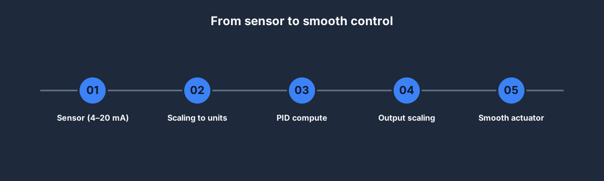
From sensor to smooth control

Every analog control loop is five steps:

  1. Sensor — a transmitter outputs 4–20 mA (industrial standard) or 0–10 V (machinery standard). Pressure, temperature, level, flow, position.
  2. Scaling — your PLC's analog input module converts mA or V to a 16-bit integer (usually 0–27648 for Siemens, 0–32767 for Rockwell, vendor-specific). Your ladder scales that to engineering units.
  3. PID compute — the PID block reads the scaled process variable (PV), compares to the setpoint (SP), and writes an output (0–100 % or scaled).
  4. Output scaling — that output is converted back to the analog output module's integer range and driven to the actuator (valve, VFD, heater).
  5. Actuator — the physical change that affects the process.

Miss any step and your loop behaves badly. Over-scale and PID thinks the PV is saturated when it's only 60%. Under-scale and the derivative term goes wild.

The scaling rung in plain terms

A 4–20 mA transmitter measuring 0–100 °C. For more worked examples of reading and scaling analog inputs in ladder logic, see analog input PLC examples.

raw_input ∈ 0..27648   (Siemens SM1231 convention)
4 mA → raw = 5530
20 mA → raw = 27648
span_raw = 27648 - 5530 = 22118
span_eu = 100 - 0 = 100

PV_in_EU := (raw_input - 5530) * 100 / 22118

Write that once in a scaling function block, call it for every analog input, and you're done. Never retype the magic numbers.

PID in plain English

Three terms. None of them are scary on their own.

  • P (Proportional) — "how far off are we?" Bigger error → bigger corrective output. If the tank is 10 °C below setpoint, open the steam valve wider.
  • I (Integral) — "how long have we been off?" Small persistent error → slowly bigger output. Corrects for steady-state offset that P alone can't fix.
  • D (Derivative) — "how fast is the error changing?" Rapid change → damping output. Prevents overshoot on fast loops; amplifies noise on slow loops. Often turned off.

In ladder logic, every vendor gives you a PID function block with these three as parameters: Kp, Ki (or Ti), Kd (or Td). You set them, the block does the math.

When PID isn't the right tool
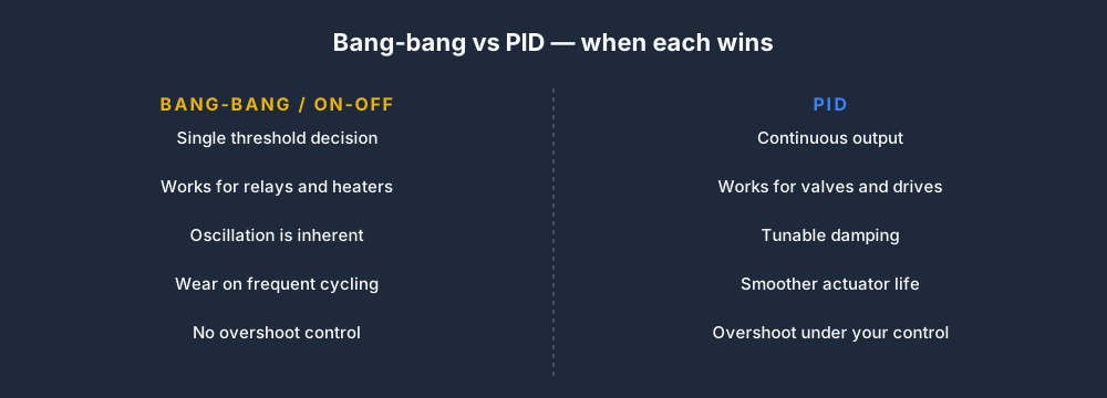
Bang-bang vs PID — when each wins

Simple on-off (bang-bang) control is often better than PID for:

  • Water heaters with big tanks — oscillation is fine, PID is overkill.
  • Cabin heaters in HVAC where setpoint drift of ±1 °C doesn't matter.
  • Relay-driven systems that can't cycle faster than once every 30 seconds.

Reserve PID for:

  • Analog actuators — modulating valves, VFDs, SCRs, servo drives.
  • Loops where overshoot matters — temperature loops on chemical reactions, pressure loops on regulators.
  • Loops where ripple matters — pressure control in process systems, level control in tank blending.

If your actuator is a contactor or a solenoid, use on-off. If it's a valve or VFD, use PID.

The 90% tuning method

The 90% tuning method (no Ziegler-Nichols drama)

Step by step, for the vast majority of temperature, level, flow, and pressure loops:

  1. Set P only. Start with Ki and Kd at 0. Pick a small Kp — 0.1 is a reasonable start for most loops.
  2. Ramp up P. Double Kp every 30 seconds (or every 2–3 settling times for slow loops) while making step changes to the setpoint. Watch the PV response.
  3. Stop when it oscillates. When the PV starts swinging back and forth around the setpoint, you've found the critical gain. Note the period of the oscillation — this is Tc, typically 10–60 seconds for temperature loops, 1–5 seconds for fast pressure loops.
  4. Halve the Kp. That's your operating P. The loop is now stable but sluggish, with steady-state offset.
  5. Add I with Ti = Tc. Set the integral time to roughly the period of oscillation. The loop now eliminates steady-state offset.
  6. Leave D at zero unless you see unacceptable overshoot on step response. If you add D, start at Td = Tc / 8 and increase cautiously.
  7. Test. Do a 10% setpoint change. Good tune: reaches setpoint in 2–3 settling times, less than 10% overshoot. If not, adjust Ki or Kd slightly.
  8. Lock in the gains. Write them down. Add a comment in the PID block noting the tuning date and who did it.

That's the whole method. It won't beat a control engineer with proper step-response identification tools, but it'll get you 90% of the way in an afternoon.

Avoiding the classic PID traps

Five things that bite newcomers:

  1. Integral windup. If your output saturates (valve fully open) and error persists, the integral keeps accumulating. When error finally reverses, the loop overshoots wildly. Cure: use vendor's anti-windup feature (all modern PID blocks have one).
  2. Derivative kick on setpoint changes. If D acts on error, a step setpoint change produces a huge derivative spike. Cure: use "D on PV only" configuration (standard on modern blocks).
  3. Scan time too slow. If your scan is 100 ms and your loop period is 1 second, you've got only 10 samples per cycle. Marginal. Move PID to a faster task or shorten your scan.
  4. Noisy PV. A shaky sensor reading amplifies D wildly. Cure: filter the PV (first-order lag, 0.1–0.5 seconds) before feeding it to the PID block.
  5. Tuning with the wrong process. If you tune a water-heating loop with the tank empty, the gains won't fit the real load. Tune with the real process running.

PID in IEC, Rockwell, Siemens

Same math, slightly different parameter names:

  • IEC 61131-3PID function block, parameters CTRL_MODE, SP_INT, PV_IN, LMN_PER (output), tuning via GAIN, TI, TD.
  • Rockwell Studio 5000PIDE (Enhanced PID) function block. Parameters Kp, Ki, Kd. Auto-tune feature built in.
  • Siemens TIA PortalPID_Compact (for S7-1200) or PID_3Step (for S7-1500). Auto-tune modes called "Pretuning" and "Fine-tuning."

Our PID Temperature scenario is a browser playground for this method — tune it until the loop settles smoothly, then port the gains to real hardware.

FAQ

Is PID hard to tune?

The 90% method above is not. Ziegler-Nichols is. Most engineers who say PID is hard were taught via Z-N without seeing the simpler iterative approach.

Do I need to learn the math?

No. You need intuition for what each term does (see "PID in plain English" above) and a systematic tuning method. The math is optional.

What's the best PID tuning software?

For most loops: none. The 90% method works with a stopwatch and the PLC's online view. For tricky loops: ExperTune PlantTriage, Matrikon Process Doctor, or vendor-specific auto-tune features.

How long does PID tuning take?

30 minutes per loop for the 90% method. 4 hours per loop if you want a professional-quality tune with step-response identification.

Do modern PLCs auto-tune PID?

Siemens PID_Compact and Rockwell PIDE both offer auto-tune. They work for about 70% of loops and are a good starting point for the other 30%.

Where to start

  1. Open our PID Temperature scenario. Pro tier.
  2. Start with Kp = 0.1, Ki = 0, Kd = 0.
  3. Follow the eight steps above.
  4. When the loop settles cleanly, port the gains to a real PID block in Studio 5000, TIA Portal, or whatever IDE your target job uses.

Eight steps, thirty minutes, one dominant practical skill. That's PID on a PLC.
ShareX / TwitterLinkedIn

From reading to running logic

Practice this yourself in the simulator

Start with guided PLC practice in your browser. No install and no credit card required.

Start practising free

Continue learning

Related field notes

All articles
pid
analogue

PID Control for PLCs: Practical Tuning Guide

Learn how PID controllers work in PLCs: proportional, integral, and derivative terms explained. Includes practical tuning methods and IEC 61131-3 code examples.

11 min read
tutorial
examples

PLC Temperature Control with a Ladder Diagram (On/Off and PID)

How PLC temperature control works, from the RTD or thermocouple input to the heater output. A worked temperature control using PLC ladder diagram, on/off vs PID, hysteresis, and a control-logic flowchart.

8 min read
tutorial
examples

PLC Pump Control Logic: Duty/Standby and Lead-Lag (Ladder Examples)

Pump control logic in a PLC explained with ladder diagrams. Start/stop on level, seal-in rungs, duty standby alternation, lead lag pump control and automatic fault changeover — with state, timing and architecture diagrams.

9 min read

Technical reference and worked-example guide

Analog I/O and PID tuning guide: implementation, evidence and troubleshooting

Direct answer

Analog I/O and PID tuning guide becomes useful when it connects process objective, pv range and unit, sensor and transmitter dynamics, input scaling, sample and filter, controller direction, output limits, actuator response, mode transfer, tuning method and acceptance metrics with process condition through sensor, transmitter, analog input, scaled pv, pid calculation, bounded output, final control element, process response and independent trend evidence, then proves a small approved test produces coherent pv and output trends and the loop meets declared response and steady-state criteria without saturation under normal, boundary, fault and recovery conditions. The objective is a repeatable engineering or learning result, not merely activity inside a page or tool.

This guide is written for pLC and process-control learners connecting transmitter range, input scaling, sample behavior and output actuation to safe, evidence-led PID tuning. The intended result is specific: the reader can prove the measurement and final-control path before tuning and can evaluate setpoint response, disturbance rejection, saturation and recovery with trends.

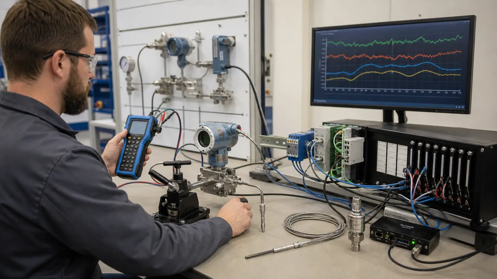
an instrumentation diagnostics bench connecting pressure, temperature and smart transmitters to isolated analog channels and time-aligned trend evidence while studying analog measurement quality and PID tuning evidence
The scene keeps analog measurement quality and PID tuning evidence connected to a declared operating condition, observable evidence, safe boundaries and a result another person can reproduce.

System map / 02

Six concepts that control the result

Treat these as connected checkpoints. Each checkpoint has an expected state, an observable state and a boundary to the next part of the system. That structure prevents a software indication from being mistaken for physical proof.

NODE 01observable

Define the operating contract

process objective, PV range and unit, sensor and transmitter dynamics, input scaling, sample and filter, controller direction, output limits, actuator response, mode transfer, tuning method and acceptance metrics. For analog measurement quality and PID tuning evidence, record the initial condition, actor, requested change, observable result and stopping condition before selecting a tool or implementation.

NODE 02observable

Map the evidence path

process condition through sensor, transmitter, analog input, scaled PV, PID calculation, bounded output, final control element, process response and independent trend evidence. Separate request, internal state, output or service, physical or user-visible result and independent feedback so each boundary can be inspected.

NODE 03observable

Prove normal operation

a small approved test produces coherent PV and output trends and the loop meets declared response and steady-state criteria without saturation. Run more than one cycle from a known state and retain the values, timings or artifacts that demonstrate repeatability.

NODE 04observable

Exercise a boundary case

wrong direction, noisy PV, bad scaling, dead time, actuator stiction, output saturation, integral windup, manual-auto transfer, sensor failure and restart. Choose minimum, maximum, simultaneous, delayed or restart conditions that reveal assumptions hidden by the happy path.

NODE 05observable

Diagnose a controlled fault

a process, sensor, loop, input, scaling, sample, controller, tuning, output, actuator or acceptance mismatch. Preserve the first symptom, divide the system at a measurable boundary and change one condition only after predicting the result.

NODE 06observable

Transfer and hand over

the loop tuned and validated on the target controller and process under approved operating limits and rollback procedures. Restore normal state, remove temporary changes, repeat affected checks and document which claims remain limited to the learning environment.

Procedure / 03

A six-step practice and commissioning workflow

Run the steps in order the first time. Later, the same structure becomes a diagnostic loop: define the expected condition, observe the boundary, interpret the difference and choose one proving action.

  1. 01

    Write the acceptance case

    Convert process objective, pv range and unit, sensor and transmitter dynamics, input scaling, sample and filter, controller direction, output limits, actuator response, mode transfer, tuning method and acceptance metrics into initial conditions, one stimulus and observable pass criteria.

    Evidence: Another person can repeat the case without guessing the intended result.

    Avoid: Using page completion or an animation as the acceptance criterion.

  2. 02

    Build the map

    Document process condition through sensor, transmitter, analog input, scaled pv, pid calculation, bounded output, final control element, process response and independent trend evidence and name who owns each state or decision.

    Evidence: Every request and result has a source, destination and useful inspection point.

    Avoid: Using the same value as command, status and independent feedback.

  3. 03

    Run the baseline

    Apply a small approved test produces coherent pv and output trends and the loop meets declared response and steady-state criteria without saturation from a clean start and record the expected evidence.

    Evidence: Repeated runs produce the same bounded result.

    Avoid: Changing several parameters before a baseline exists.

  4. 04

    Challenge assumptions

    Test wrong direction, noisy pv, bad scaling, dead time, actuator stiction, output saturation, integral windup, manual-auto transfer, sensor failure and restart without changing the acceptance contract.

    Evidence: Limits, timing and restart behavior reach defined states.

    Avoid: Testing only one ideal sequence.

  5. 05

    Isolate one failure

    Introduce or analyse a process, sensor, loop, input, scaling, sample, controller, tuning, output, actuator or acceptance mismatch and locate the first disagreement.

    Evidence: The proving action distinguishes the leading hypotheses.

    Avoid: Resetting, forcing or replacing before evidence is retained.

  6. 06

    Close the evidence loop

    Complete the loop tuned and validated on the target controller and process under approved operating limits and rollback procedures and repeat the affected regression cases.

    Evidence: Reference use is complete when inputs, assumptions, units or initial conditions are recorded and the result is independently checked at a useful boundary.

    Avoid: Treating an acknowledged message or one successful rerun as handover.

Diagnostic matrix / 04

Symptoms, proving points and next actions

The table is a reasoning aid, not a parts-replacement chart. Preserve the initial symptom, inspect the named boundary and use the interpretation to choose the next controlled test. Site safety procedures and equipment manuals remain authoritative.

Diagnostic symptoms, inspection points, interpretations and next actions for Analog I/O and PID tuning guide: implementation, evidence and troubleshooting
Observed symptomInspectInterpretationNext proving action
The expected result is unclearRequirement, initial state, actor, stimulus, units and pass conditionThe technician, programmer and reviewer may be solving different versions of the task.Rewrite one observable acceptance case before continuing.
Internal state changes but the outcome does notRequest, final owner, output or service boundary and independent feedbackA software or interface indication proves intent at one layer, not the complete outcome.Trace the first boundary after the changing state.
Normal case passes but an edge case failsLimits, timing, simultaneous events, reset and restart assumptionsThe implementation contains a hidden assumption exposed by the changed condition.Add the failed boundary as a permanent regression case.
The failure disappears after resetOriginal symptom, histories, diagnostics, timestamps and active causeReset changed evidence or state without proving the initiating cause.Reproduce under a controlled condition and preserve pre/post-event data.
Simulator and target disagreeModel boundary, software version, task timing, I/O behavior, data types and configurationA learning model and the intended target do not share one of the recorded assumptions.Reduce the case and verify against current target documentation.
The result cannot be explainedPrediction, observation, proving action, alternative hypotheses and limitationsActivity occurred but the evidence is not yet transferable or reviewable.Have the learner defend the signal path and repeat a changed case.

Product evidence / 05

What the browser practice can actually demonstrate

The page connects definitions and worked examples to runnable tools, explicit assumptions and repeatable checks so a formula or pattern can be challenged.

Where simulation stops

A generic guide cannot prescribe tuning for an unknown process, validate safety or equipment limits, or replace target-controller algorithms, process expertise and supervised commissioning.

Commissioning notebook / 06

Six cases that turn the concepts into evidence

Use these as written briefs rather than click-through instructions. For every case, state the expected condition before acting, retain the first useful observation and explain why the final result proves the requirement. A different program or component choice can still be correct when it produces the same bounded behavior and evidence.

Case 01

predict → observe → prove

Prove define the operating contract

Engineering context. process objective, PV range and unit, sensor and transmitter dynamics, input scaling, sample and filter, controller direction, output limits, actuator response, mode transfer, tuning method and acceptance metrics. For analog measurement quality and PID tuning evidence, record the initial condition, actor, requested change, observable result and stopping condition before selecting a tool or implementation. Begin with a written normal condition and identify which request, state, physical result or communication value will provide independent confirmation. Do not begin by changing the configuration; the initial state is part of the evidence and should remain reproducible.

Controlled setup. Use the “Write the acceptance case” stage of the workflow: convert process objective, pv range and unit, sensor and transmitter dynamics, input scaling, sample and filter, controller direction, output limits, actuator response, mode transfer, tuning method and acceptance metrics into initial conditions, one stimulus and observable pass criteria. The acceptance record should show this result: another person can repeat the case without guessing the intended result. Record initial conditions, the exact stimulus and the observation point so another learner can repeat the case without relying on your memory.

Fault challenge. Introduce or analyse “The expected result is unclear” as one bounded deviation. Inspect requirement, initial state, actor, stimulus, units and pass condition The working interpretation is that the technician, programmer and reviewer may be solving different versions of the task. The next proving action is to rewrite one observable acceptance case before continuing. Change only one condition before observing the result, and preserve timestamps or measurements where timing matters.

Review and recovery. The most common trap here is using page completion or an animation as the acceptance criterion. After restoring the cause, repeat the normal case and at least one stop, timeout, disconnect or restart boundary relevant to this topic. Remove temporary forces and bypasses, return the model to a known state and retain the evidence that both operation and recovery are deliberate.

Explain it aloud: Should I tune PID before checking analog scaling? A defensible short answer is: No. Prove sensor range, loop signal, raw input, engineering units, controller direction and final-element response before changing tuning constants.

Case 02

predict → observe → prove

Prove map the evidence path

Engineering context. process condition through sensor, transmitter, analog input, scaled PV, PID calculation, bounded output, final control element, process response and independent trend evidence. Separate request, internal state, output or service, physical or user-visible result and independent feedback so each boundary can be inspected. Begin with a written normal condition and identify which request, state, physical result or communication value will provide independent confirmation. Do not begin by changing the configuration; the initial state is part of the evidence and should remain reproducible.

Controlled setup. Use the “Build the map” stage of the workflow: document process condition through sensor, transmitter, analog input, scaled pv, pid calculation, bounded output, final control element, process response and independent trend evidence and name who owns each state or decision. The acceptance record should show this result: every request and result has a source, destination and useful inspection point. Record initial conditions, the exact stimulus and the observation point so another learner can repeat the case without relying on your memory.

Fault challenge. Introduce or analyse “Internal state changes but the outcome does not” as one bounded deviation. Inspect request, final owner, output or service boundary and independent feedback The working interpretation is that a software or interface indication proves intent at one layer, not the complete outcome. The next proving action is to trace the first boundary after the changing state. Change only one condition before observing the result, and preserve timestamps or measurements where timing matters.

Review and recovery. The most common trap here is using the same value as command, status and independent feedback. After restoring the cause, repeat the normal case and at least one stop, timeout, disconnect or restart boundary relevant to this topic. Remove temporary forces and bypasses, return the model to a known state and retain the evidence that both operation and recovery are deliberate.

Explain it aloud: What data is useful for PID tuning? A defensible short answer is: Trend timestamped setpoint, process value, controller output, mode, limits and relevant disturbances at a rate that exposes the process dynamics.

Case 03

predict → observe → prove

Prove prove normal operation

Engineering context. a small approved test produces coherent PV and output trends and the loop meets declared response and steady-state criteria without saturation. Run more than one cycle from a known state and retain the values, timings or artifacts that demonstrate repeatability. Begin with a written normal condition and identify which request, state, physical result or communication value will provide independent confirmation. Do not begin by changing the configuration; the initial state is part of the evidence and should remain reproducible.

Controlled setup. Use the “Run the baseline” stage of the workflow: apply a small approved test produces coherent pv and output trends and the loop meets declared response and steady-state criteria without saturation from a clean start and record the expected evidence. The acceptance record should show this result: repeated runs produce the same bounded result. Record initial conditions, the exact stimulus and the observation point so another learner can repeat the case without relying on your memory.

Fault challenge. Introduce or analyse “Normal case passes but an edge case fails” as one bounded deviation. Inspect limits, timing, simultaneous events, reset and restart assumptions The working interpretation is that the implementation contains a hidden assumption exposed by the changed condition. The next proving action is to add the failed boundary as a permanent regression case. Change only one condition before observing the result, and preserve timestamps or measurements where timing matters.

Review and recovery. The most common trap here is changing several parameters before a baseline exists. After restoring the cause, repeat the normal case and at least one stop, timeout, disconnect or restart boundary relevant to this topic. Remove temporary forces and bypasses, return the model to a known state and retain the evidence that both operation and recovery are deliberate.

Explain it aloud: What should I learn first about analog measurement quality and PID tuning evidence? A defensible short answer is: Start with the operating contract and evidence path: process objective, pv range and unit, sensor and transmitter dynamics, input scaling, sample and filter, controller direction, output limits, actuator response, mode transfer, tuning method and acceptance metrics, followed by process condition through sensor, transmitter, analog input, scaled pv, pid calculation, bounded output, final control element, process response and independent trend evidence. Add advanced features only after the baseline is predictable.

Case 04

predict → observe → prove

Prove exercise a boundary case

Engineering context. wrong direction, noisy PV, bad scaling, dead time, actuator stiction, output saturation, integral windup, manual-auto transfer, sensor failure and restart. Choose minimum, maximum, simultaneous, delayed or restart conditions that reveal assumptions hidden by the happy path. Begin with a written normal condition and identify which request, state, physical result or communication value will provide independent confirmation. Do not begin by changing the configuration; the initial state is part of the evidence and should remain reproducible.

Controlled setup. Use the “Challenge assumptions” stage of the workflow: test wrong direction, noisy pv, bad scaling, dead time, actuator stiction, output saturation, integral windup, manual-auto transfer, sensor failure and restart without changing the acceptance contract. The acceptance record should show this result: limits, timing and restart behavior reach defined states. Record initial conditions, the exact stimulus and the observation point so another learner can repeat the case without relying on your memory.

Fault challenge. Introduce or analyse “The failure disappears after reset” as one bounded deviation. Inspect original symptom, histories, diagnostics, timestamps and active cause The working interpretation is that reset changed evidence or state without proving the initiating cause. The next proving action is to reproduce under a controlled condition and preserve pre/post-event data. Change only one condition before observing the result, and preserve timestamps or measurements where timing matters.

Review and recovery. The most common trap here is testing only one ideal sequence. After restoring the cause, repeat the normal case and at least one stop, timeout, disconnect or restart boundary relevant to this topic. Remove temporary forces and bypasses, return the model to a known state and retain the evidence that both operation and recovery are deliberate.

Explain it aloud: How do I practise analog measurement quality and PID tuning evidence effectively? A defensible short answer is: Use short cases with known initial conditions, a written prediction, one action and an observable result. Then alter a boundary or fault and explain why the evidence changed.

Case 05

predict → observe → prove

Prove diagnose a controlled fault

Engineering context. a process, sensor, loop, input, scaling, sample, controller, tuning, output, actuator or acceptance mismatch. Preserve the first symptom, divide the system at a measurable boundary and change one condition only after predicting the result. Begin with a written normal condition and identify which request, state, physical result or communication value will provide independent confirmation. Do not begin by changing the configuration; the initial state is part of the evidence and should remain reproducible.

Controlled setup. Use the “Isolate one failure” stage of the workflow: introduce or analyse a process, sensor, loop, input, scaling, sample, controller, tuning, output, actuator or acceptance mismatch and locate the first disagreement. The acceptance record should show this result: the proving action distinguishes the leading hypotheses. Record initial conditions, the exact stimulus and the observation point so another learner can repeat the case without relying on your memory.

Fault challenge. Introduce or analyse “Simulator and target disagree” as one bounded deviation. Inspect model boundary, software version, task timing, I/O behavior, data types and configuration The working interpretation is that a learning model and the intended target do not share one of the recorded assumptions. The next proving action is to reduce the case and verify against current target documentation. Change only one condition before observing the result, and preserve timestamps or measurements where timing matters.

Review and recovery. The most common trap here is resetting, forcing or replacing before evidence is retained. After restoring the cause, repeat the normal case and at least one stop, timeout, disconnect or restart boundary relevant to this topic. Remove temporary forces and bypasses, return the model to a known state and retain the evidence that both operation and recovery are deliberate.

Explain it aloud: What counts as proof of competence? A defensible short answer is: A repeatable artifact or system result plus an explanation of the signal path is stronger than time spent, screenshots or a copied answer. Physical competence requires separate supervised evidence.

Case 06

predict → observe → prove

Prove transfer and hand over

Engineering context. the loop tuned and validated on the target controller and process under approved operating limits and rollback procedures. Restore normal state, remove temporary changes, repeat affected checks and document which claims remain limited to the learning environment. Begin with a written normal condition and identify which request, state, physical result or communication value will provide independent confirmation. Do not begin by changing the configuration; the initial state is part of the evidence and should remain reproducible.

Controlled setup. Use the “Close the evidence loop” stage of the workflow: complete the loop tuned and validated on the target controller and process under approved operating limits and rollback procedures and repeat the affected regression cases. The acceptance record should show this result: reference use is complete when inputs, assumptions, units or initial conditions are recorded and the result is independently checked at a useful boundary. Record initial conditions, the exact stimulus and the observation point so another learner can repeat the case without relying on your memory.

Fault challenge. Introduce or analyse “The result cannot be explained” as one bounded deviation. Inspect prediction, observation, proving action, alternative hypotheses and limitations The working interpretation is that activity occurred but the evidence is not yet transferable or reviewable. The next proving action is to have the learner defend the signal path and repeat a changed case. Change only one condition before observing the result, and preserve timestamps or measurements where timing matters.

Review and recovery. The most common trap here is treating an acknowledged message or one successful rerun as handover. After restoring the cause, repeat the normal case and at least one stop, timeout, disconnect or restart boundary relevant to this topic. Remove temporary forces and bypasses, return the model to a known state and retain the evidence that both operation and recovery are deliberate.

Explain it aloud: Why test faults and restart behavior? A defensible short answer is: Because a process, sensor, loop, input, scaling, sample, controller, tuning, output, actuator or acceptance mismatch or wrong direction, noisy pv, bad scaling, dead time, actuator stiction, output saturation, integral windup, manual-auto transfer, sensor failure and restart can expose assumptions that never appear during ideal startup and steady operation.

Answer surface / 07

Questions people ask about Analog I/O and PID tuning guide

These concise answers define the operating, training and product boundaries most often missed in broad summaries. The full workflow and diagnostic table above provide the evidence behind them.

Should I tune PID before checking analog scaling?

No. Prove sensor range, loop signal, raw input, engineering units, controller direction and final-element response before changing tuning constants.

What data is useful for PID tuning?

Trend timestamped setpoint, process value, controller output, mode, limits and relevant disturbances at a rate that exposes the process dynamics.

What should I learn first about analog measurement quality and PID tuning evidence?

Start with the operating contract and evidence path: process objective, pv range and unit, sensor and transmitter dynamics, input scaling, sample and filter, controller direction, output limits, actuator response, mode transfer, tuning method and acceptance metrics, followed by process condition through sensor, transmitter, analog input, scaled pv, pid calculation, bounded output, final control element, process response and independent trend evidence. Add advanced features only after the baseline is predictable.

How do I practise analog measurement quality and PID tuning evidence effectively?

Use short cases with known initial conditions, a written prediction, one action and an observable result. Then alter a boundary or fault and explain why the evidence changed.

What counts as proof of competence?

A repeatable artifact or system result plus an explanation of the signal path is stronger than time spent, screenshots or a copied answer. Physical competence requires separate supervised evidence.

Why test faults and restart behavior?

Because a process, sensor, loop, input, scaling, sample, controller, tuning, output, actuator or acceptance mismatch or wrong direction, noisy pv, bad scaling, dead time, actuator stiction, output saturation, integral windup, manual-auto transfer, sensor failure and restart can expose assumptions that never appear during ideal startup and steady operation.

Can browser practice replace official software or hardware?

No. It can build concepts and diagnostic reasoning. Exact firmware, I/O electrical behavior, networking, safety and commissioning require current official tools, documentation and target equipment.

How should progress be documented?

Keep the requirement, initial state, program or configuration, observed values, fault hypothesis, proving action, recovery result and a concise limitations statement.