Prove the loop before scaling
Confirm supply, polarity, series connection and input-card mode. A perfect scaling equation cannot fix an open loop or a voltage input configured for current.
Scale a real 4–20 mA signal, diagnose a broken loop and build calibration evidence before working on live process instrumentation.
First challenge
Scale a 4–20 mA transmitter
Convert a loop current into engineering units for a configurable transmitter range.
Reusable lab resources
Calibration record templateCSVRecognise the complete signal path
A current-loop calculation only becomes useful when you can connect it to the power supply, instrument, input channel, engineering range and process response. These six views follow that workflow from the bench to the plant.
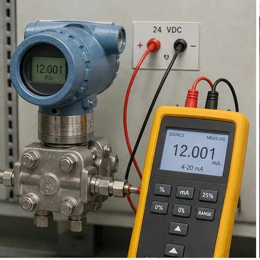
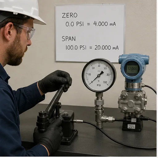
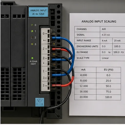
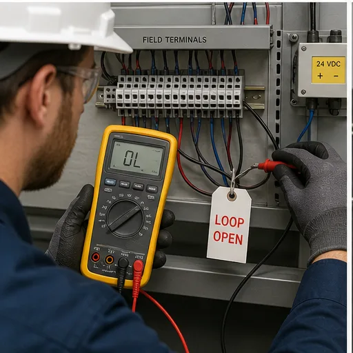
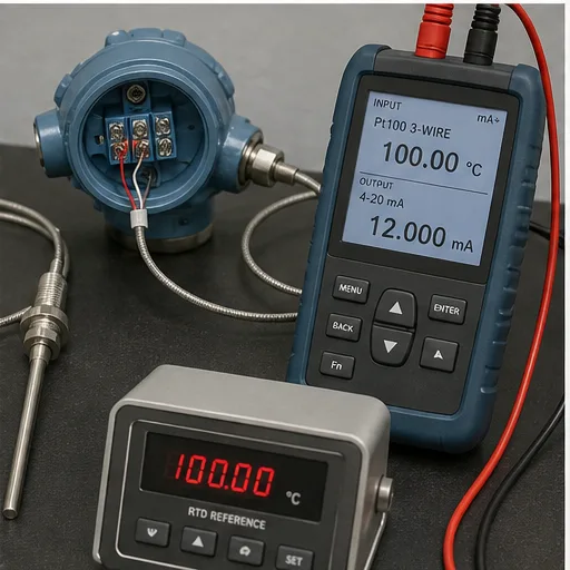
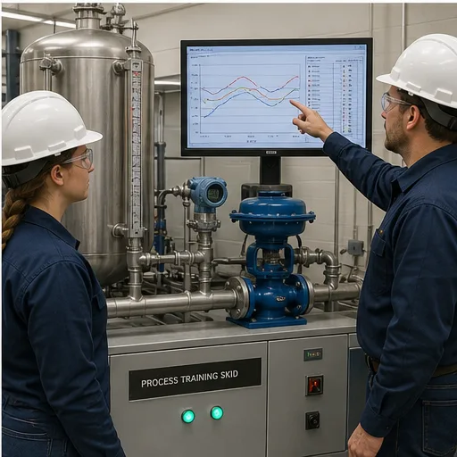
Interactive calibration lab
Convert a loop current into engineering units for a configurable transmitter range.
The backend calculates the expected result and returns individual checks, a score and reproducible evidence. Client-supplied scores are ignored.
Your run is free. Keep the evidence when it matters.
Create an account only when you want saved attempts, projects, sharing and progress.
Training outcomes
Each run teaches a transferable industrial workflow and produces evidence you can inspect, repeat and discuss.
Convert loop current into pressure, temperature, flow or level units.
Explain live zero and separate a true zero measurement from a broken loop.
Build a repeatable calibration record with objective grading.
Move directly into PLC analog-I/O and process-control scenarios.
Field method
Confirm supply, polarity, series connection and input-card mode. A perfect scaling equation cannot fix an open loop or a voltage input configured for current.
For a standard loop, percent span is (mA − 4) ÷ 16. Multiply that fraction by the engineering span and add the engineering minimum.
A defensible calibration records the test points, reference standard, tolerance, adjustment and final result—not just a pass tick.
Continue from a single exercise to a complete training record.
Guided scenarios, saved progress, fault diagnosis and instructor reporting are built into the main platform.
Technical practice library
Each reference explains a distinct industrial task and links back to an exact grader preset with server-owned acceptance evidence.
Gauge pressure transmitter
Calculate and grade a 0–10 bar pressure-transmitter signal at 12 mA, then record the calibration evidence and live-zero checks.
RTD temperature transmitter
Work a bipolar temperature-transmitter scaling example at 8 mA and verify the result in a server-graded instrumentation lab.
Hydrostatic level transmitter
Convert a 16 mA level signal into metres, verify 75% span and carry the evidence into the instrumentation simulator.
Magnetic flow transmitter
Calculate an 80 m³/h flow indication from 10.4 mA and validate the linear scaling in the browser lab.
Control-valve position transmitter
Translate 18.4 mA into 90% valve travel and separate feedback scaling from the output command.
Vacuum pressure transmitter
Solve a negative-range 4–20 mA vacuum-transmitter example at 6.4 mA and verify the −85 kPa result with graded evidence.
Low-range differential-pressure transmitter
Calculate a 160 Pa filter differential from 14.24 mA and verify the air-handler alarm input scaling in the graded lab.
Conductivity transmitter
Convert 7.2 mA into 4 mS/cm and validate the analogue scaling used by a water-quality interlock.
Technical review
Reviewed 7 August 2026. The simulator teaches a repeatable training method; always use the exact module and instrument manuals for live commissioning work.
Instrumentation loop field guide
Direct answer
Instrumentation simulation should connect the physical variable, sensor, transmitter range, loop signal, input channel, raw counts, engineering scaling, quality and control response. Calibration and troubleshooting need known inputs and evidence at each boundary.
This guide is written for instrumentation learners, maintenance technicians and PLC programmers working with pressure, temperature, level, flow and 4–20 mA signals. The intended result is specific: the learner can configure a measurement contract, perform zero/mid/span checks, diagnose open or mis-scaled loops and distinguish sensor, transmitter, wiring, input and software faults.
System map / 02
Treat these as connected checkpoints. Each checkpoint has an expected state, an observable state and a boundary to the next part of the system. That structure prevents a software indication from being mistaken for physical proof.
Lower and upper range values define the engineering quantity represented by the signal.
A 4–20 mA loop separates live zero from full scale and requires compatible supply, burden and input configuration.
The module converts electrical signal into counts; software then maps counts into units with range and fault policy.
Sensor, transmitter, wiring, input and scaling each contribute uncertainty or error.
A numeric value needs validity, timestamp and fault state; a frozen plausible number can be dangerous.
Known inputs, as-found/as-left results and adjustment decisions make the outcome reproducible.
Procedure / 03
Run the steps in order the first time. Later, the same structure becomes a diagnostic loop: define the expected condition, observe the boundary, interpret the difference and choose one proving action.
State variable, units, range and required accuracy.
Evidence: The loop has an engineering contract.
Avoid: Starting from a PLC raw range.
Map sensor, transmitter, supply, terminals, input and scaling.
Evidence: Every boundary is named.
Avoid: Treating the transmitter and sensor as one mystery device.
Use safe low, midpoint and high references.
Evidence: Input and display can be compared at each point.
Avoid: Adjusting from one point.
Capture signal and engineering value before adjustment.
Evidence: The original error is preserved.
Avoid: Erasing evidence by zeroing immediately.
Correct zero or span only according to the device method.
Evidence: All points improve within the intended tolerance.
Avoid: Using PLC scaling to hide transmitter error.
Open, drive out of range or freeze the modeled signal.
Evidence: Quality and control response are observable.
Avoid: Testing only nominal calibration.
Diagnostic matrix / 04
The table is a reasoning aid, not a parts-replacement chart. Preserve the initial symptom, inspect the named boundary and use the interpretation to choose the next controlled test. Site safety procedures and equipment manuals remain authoritative.
| Observed symptom | Inspect | Interpretation | Next proving action |
|---|---|---|---|
| Zero offset | Applied reference, transmitter zero, loop current and software lower range | A constant error suggests an offset at one layer. | Compare current and raw counts. |
| Span error | High reference, transmitter span, input range and scaling slope | Error grows across range. | Check at least three points. |
| Fixed low value | Supply, open loop, polarity, input mode and underrange handling | The loop may be open or unpowered. | Measure current safely. |
| Plausible wrong value | Units, configured range and scaling endpoints | The electrical loop can be healthy with wrong engineering mapping. | Verify the range contract. |
| Noisy trend | Process variation, grounding, shielding, filtering and sampling | Noise source may be physical or acquisition related. | Compare signal at successive boundaries. |
| Frozen value | Timestamp, quality, communication and update state | A valid-looking number may be stale. | Require freshness detection. |
Product evidence / 05
The browser lab combines transmitters, loop values, PLC scaling, process trends and controlled faults with related analog scenarios.
The model does not replace a traceable calibrator, hazardous-area procedure, exact transmitter manual, process isolation or site calibration record.
Commissioning notebook / 06
Use these as written briefs rather than click-through instructions. For every case, state the expected condition before acting, retain the first useful observation and explain why the final result proves the requirement. A different program or component choice can still be correct when it produces the same bounded behavior and evidence.
Case 01
predict → observe → prove
Engineering context. Lower and upper range values define the engineering quantity represented by the signal. Begin with a written normal condition and identify which request, state, physical result or communication value will provide independent confirmation. Do not begin by changing the configuration; the initial state is part of the evidence and should remain reproducible.
Controlled setup. Use the “Define the measurand” stage of the workflow: state variable, units, range and required accuracy. The acceptance record should show this result: the loop has an engineering contract. Record initial conditions, the exact stimulus and the observation point so another learner can repeat the case without relying on your memory.
Fault challenge. Introduce or analyse “Zero offset” as one bounded deviation. Inspect applied reference, transmitter zero, loop current and software lower range The working interpretation is that a constant error suggests an offset at one layer. The next proving action is to compare current and raw counts. Change only one condition before observing the result, and preserve timestamps or measurements where timing matters.
Review and recovery. The most common trap here is starting from a PLC raw range. After restoring the cause, repeat the normal case and at least one stop, timeout, disconnect or restart boundary relevant to this topic. Remove temporary forces and bypasses, return the model to a known state and retain the evidence that both operation and recovery are deliberate.
Explain it aloud: What is an instrumentation simulator? A defensible short answer is: It models measurement devices, loop signals, scaling and process response so learners can calibrate and diagnose without a live plant.
Case 02
predict → observe → prove
Engineering context. A 4–20 mA loop separates live zero from full scale and requires compatible supply, burden and input configuration. Begin with a written normal condition and identify which request, state, physical result or communication value will provide independent confirmation. Do not begin by changing the configuration; the initial state is part of the evidence and should remain reproducible.
Controlled setup. Use the “Review the loop” stage of the workflow: map sensor, transmitter, supply, terminals, input and scaling. The acceptance record should show this result: every boundary is named. Record initial conditions, the exact stimulus and the observation point so another learner can repeat the case without relying on your memory.
Fault challenge. Introduce or analyse “Span error” as one bounded deviation. Inspect high reference, transmitter span, input range and scaling slope The working interpretation is that error grows across range. The next proving action is to check at least three points. Change only one condition before observing the result, and preserve timestamps or measurements where timing matters.
Review and recovery. The most common trap here is treating the transmitter and sensor as one mystery device. After restoring the cause, repeat the normal case and at least one stop, timeout, disconnect or restart boundary relevant to this topic. Remove temporary forces and bypasses, return the model to a known state and retain the evidence that both operation and recovery are deliberate.
Explain it aloud: Why does 4 mA represent zero? A defensible short answer is: It provides a live-zero signal that can be distinguished from some open-circuit conditions while reserving 20 mA for the upper range.
Case 03
predict → observe → prove
Engineering context. The module converts electrical signal into counts; software then maps counts into units with range and fault policy. Begin with a written normal condition and identify which request, state, physical result or communication value will provide independent confirmation. Do not begin by changing the configuration; the initial state is part of the evidence and should remain reproducible.
Controlled setup. Use the “Apply known points” stage of the workflow: use safe low, midpoint and high references. The acceptance record should show this result: input and display can be compared at each point. Record initial conditions, the exact stimulus and the observation point so another learner can repeat the case without relying on your memory.
Fault challenge. Introduce or analyse “Fixed low value” as one bounded deviation. Inspect supply, open loop, polarity, input mode and underrange handling The working interpretation is that the loop may be open or unpowered. The next proving action is to measure current safely. Change only one condition before observing the result, and preserve timestamps or measurements where timing matters.
Review and recovery. The most common trap here is adjusting from one point. After restoring the cause, repeat the normal case and at least one stop, timeout, disconnect or restart boundary relevant to this topic. Remove temporary forces and bypasses, return the model to a known state and retain the evidence that both operation and recovery are deliberate.
Explain it aloud: How do you scale 4–20 mA in a PLC? A defensible short answer is: Map the configured raw low/high counts to engineering low/high values, then test endpoints, midpoint and fault ranges.
Case 04
predict → observe → prove
Engineering context. Sensor, transmitter, wiring, input and scaling each contribute uncertainty or error. Begin with a written normal condition and identify which request, state, physical result or communication value will provide independent confirmation. Do not begin by changing the configuration; the initial state is part of the evidence and should remain reproducible.
Controlled setup. Use the “Record as-found” stage of the workflow: capture signal and engineering value before adjustment. The acceptance record should show this result: the original error is preserved. Record initial conditions, the exact stimulus and the observation point so another learner can repeat the case without relying on your memory.
Fault challenge. Introduce or analyse “Plausible wrong value” as one bounded deviation. Inspect units, configured range and scaling endpoints The working interpretation is that the electrical loop can be healthy with wrong engineering mapping. The next proving action is to verify the range contract. Change only one condition before observing the result, and preserve timestamps or measurements where timing matters.
Review and recovery. The most common trap here is erasing evidence by zeroing immediately. After restoring the cause, repeat the normal case and at least one stop, timeout, disconnect or restart boundary relevant to this topic. Remove temporary forces and bypasses, return the model to a known state and retain the evidence that both operation and recovery are deliberate.
Explain it aloud: What is zero and span calibration? A defensible short answer is: Zero adjusts the lower response while span adjusts the slope or upper response; exact procedures depend on the instrument.
Case 05
predict → observe → prove
Engineering context. A numeric value needs validity, timestamp and fault state; a frozen plausible number can be dangerous. Begin with a written normal condition and identify which request, state, physical result or communication value will provide independent confirmation. Do not begin by changing the configuration; the initial state is part of the evidence and should remain reproducible.
Controlled setup. Use the “Adjust deliberately” stage of the workflow: correct zero or span only according to the device method. The acceptance record should show this result: all points improve within the intended tolerance. Record initial conditions, the exact stimulus and the observation point so another learner can repeat the case without relying on your memory.
Fault challenge. Introduce or analyse “Noisy trend” as one bounded deviation. Inspect process variation, grounding, shielding, filtering and sampling The working interpretation is that noise source may be physical or acquisition related. The next proving action is to compare signal at successive boundaries. Change only one condition before observing the result, and preserve timestamps or measurements where timing matters.
Review and recovery. The most common trap here is using PLC scaling to hide transmitter error. After restoring the cause, repeat the normal case and at least one stop, timeout, disconnect or restart boundary relevant to this topic. Remove temporary forces and bypasses, return the model to a known state and retain the evidence that both operation and recovery are deliberate.
Explain it aloud: Should scaling correct a bad transmitter? A defensible short answer is: No. Establish whether error belongs to the instrument, loop/input or software contract before changing scaling.
Case 06
predict → observe → prove
Engineering context. Known inputs, as-found/as-left results and adjustment decisions make the outcome reproducible. Begin with a written normal condition and identify which request, state, physical result or communication value will provide independent confirmation. Do not begin by changing the configuration; the initial state is part of the evidence and should remain reproducible.
Controlled setup. Use the “Test faults” stage of the workflow: open, drive out of range or freeze the modeled signal. The acceptance record should show this result: quality and control response are observable. Record initial conditions, the exact stimulus and the observation point so another learner can repeat the case without relying on your memory.
Fault challenge. Introduce or analyse “Frozen value” as one bounded deviation. Inspect timestamp, quality, communication and update state The working interpretation is that a valid-looking number may be stale. The next proving action is to require freshness detection. Change only one condition before observing the result, and preserve timestamps or measurements where timing matters.
Review and recovery. The most common trap here is testing only nominal calibration. After restoring the cause, repeat the normal case and at least one stop, timeout, disconnect or restart boundary relevant to this topic. Remove temporary forces and bypasses, return the model to a known state and retain the evidence that both operation and recovery are deliberate.
Explain it aloud: What is an as-found reading? A defensible short answer is: It is the measured condition before adjustment, retained to show drift and support maintenance decisions.
Answer surface / 07
These concise answers define the operating, training and product boundaries most often missed in broad summaries. The full workflow and diagnostic table above provide the evidence behind them.
It models measurement devices, loop signals, scaling and process response so learners can calibrate and diagnose without a live plant.
It provides a live-zero signal that can be distinguished from some open-circuit conditions while reserving 20 mA for the upper range.
Map the configured raw low/high counts to engineering low/high values, then test endpoints, midpoint and fault ranges.
Zero adjusts the lower response while span adjusts the slope or upper response; exact procedures depend on the instrument.
No. Establish whether error belongs to the instrument, loop/input or software contract before changing scaling.
It is the measured condition before adjustment, retained to show drift and support maintenance decisions.
Use input diagnostics and measured current under an approved procedure; define how underrange and bad quality propagate.
No. Formal calibration needs traceable equipment, procedures and records tied to the actual instrument.
Continue the signal path / 08