PLC Simulator
PLC Timer instructions

PLC Timers Explained: TON, TOF, TP and RTO (with Live Examples)

The four timer instructions every PLC programmer needs — on-delay, off-delay, pulse and retentive — with timing diagrams, ladder rungs, real application examples, and a browser simulator where you can watch them run.

Join 9000+ learners practicing PLC programming

Foundations

What is a PLC timer?

A PLC timer is a software instruction that measures elapsed time and controls an output bit based on whether the measured time has reached a configured threshold. Unlike a mechanical or electronic timer relay, a PLC timer exists entirely in the controller's memory — there are no physical contacts to wear out, no coil to burn, and the preset value is a number you can change from an HMI or SCADA without rewiring anything.

Every PLC timer — regardless of brand or dialect — has at least three parameters: a preset time (PT / PRE), an accumulated time (ET / ACC), and one or more status bits. Understanding these three elements is the foundation for everything else.

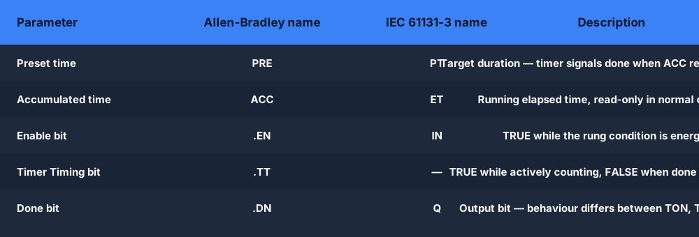
Preset time (PT / PRE). The target duration. When ACC reaches PRE, the timer signals completion. You enter PT in time units — milliseconds, seconds, or tenths of a second depending on the PLC's timebase. In Allen-Bradley Logix, PT is specified in milliseconds (e.g. T#5s or 5000 ms). In Siemens TIA Portal, you use IEC time literals (T#5S). In RSLogix 500 / SLC-500, PRE is an integer in timebase ticks.

Accumulated time (ET / ACC). The running total of time the timer has been enabled. The PLC's operating system increments ACC every scan cycle while the enable rung is TRUE. Reading ACC in your logic lets you create sub-preset triggers — for example, start a warning light at 80 % of the preset before the final done signal.

Status bits. The bits you actually use in your logic to act on the timer's state. The standard set is:

  • .EN / EN — Enable bit. TRUE whenever the rung condition is TRUE and the timer is running (or done).
  • .TT / TT — Timer Timing bit. TRUE while the timer is actively counting, FALSE once DN is set or once the rung goes FALSE.
  • .DN / Q — Done bit (Allen-Bradley .DN; IEC Q). The bit your output logic usually reads. Behaviour differs between timer types — this is the key difference between TON, TOF, TP, and RTO.
  • .PRE / PT — Readable preset value. You can address this to compare or modify the preset dynamically.
  • .ACC / ET — Readable accumulator. Use it to display progress or create cascaded timing logic.

Timebase matters for inter-operability. Most modern PLCs use a 1 ms or 10 ms system timebase for timers, but legacy platforms (Mitsubishi FX, Omron CPM) use 100 ms timers as the default. Always check your hardware manual: a PRE of 50 on a 100 ms timebase is 5 seconds, but 50 ms on a 1 ms timebase. The IEC 61131-3 standard avoids this ambiguity by requiring time literals (T#5S, T#500MS) rather than raw integers.

PLC timer instruction parameters preset accumulator bits table
Every PLC timer shares the same three core parameters — preset, accumulator, and status bits — regardless of brand.
PLC TON timer animation — the accumulated time (ACC / ET) bar ramps up toward the preset (PRE / PT) and the done (DN / Q) bit turns on the instant the accumulator reaches the presetA TON on-delay timer: the accumulated time bar ramps up toward the preset value, and the done (DN) bit turns on when the accumulator reaches preset.TONPRE 5000ACCACC ramps to PREPREDNdone bit
A timer in motion: ACC ramps toward PRE, and the DN bit fires the moment the accumulator reaches the preset.
PLC scan cycle and timers — every scan reads inputs, solves logic and updates each timer accumulator by the elapsed scan time, then writes outputs, which is why timer accuracy depends on the system timebaseThe repeating PLC scan cycle: read inputs, execute the ladder logic, update outputs, then housekeeping, looping continuously.1Read Inputs2Execute Logic3Update Outputs4HousekeepingSCANCYCLE
Why timers tick: the PLC updates every timer accumulator once per scan cycle, against the system timebase.

On-delay timer

TON — on-delay timer

The TON (on-delay timer) is the most common PLC timer instruction. It delays the activation of an output — the done bit does not turn on until the rung has been continuously TRUE for the full preset duration.

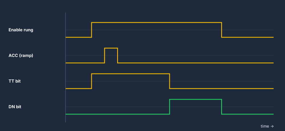
How it works, step by step. When the enable rung goes TRUE, EN is set, TT is set, and ACC begins incrementing from zero each scan. When ACC reaches PRE, DN is set and TT is cleared. If the rung goes FALSE at any point before ACC reaches PRE, EN, TT and ACC all reset to zero immediately — the timer has no memory of partial timing. If the rung goes FALSE after DN is already set, DN also clears and ACC resets.

This "forgets immediately if interrupted" behaviour is the defining characteristic of TON — and the key reason you use RTO instead when run time must accumulate across interruptions.

TON on-delay timer timing diagram ladder logic
TON timing: DN turns on only after ACC reaches PRE. If the rung drops FALSE before PRE, ACC resets to zero.
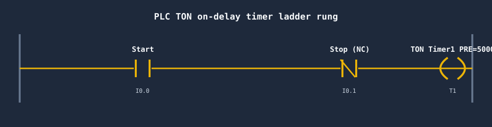
PLC TON timer ladder rung example with preset and done bit
A TON rung: a Start contact enables the timer; the Timer1.DN bit drives the output contactor only after the preset delay.
TON on-delay timer ladder rung — a Start contact enabling a TON timer block whose done (DN) bit then drives the output coil only after the preset time has elapsedA basic ladder logic rung between two power rails: an examine-if-closed contact (XIC) in series driving an output coil (OTE).L1L2] [StartXIC I:0/0LampOTE O:0/0
The TON rung in ladder form: the enable contact feeds the timer, and the DN bit gates the output coil.

Real-world uses of the TON timer

Motor start delay. Large motors draw high inrush current at startup. A TON of 3–5 seconds between energising the contactor and enabling downstream equipment (conveyors, pumps, fans) gives the motor time to reach running speed and current to stabilise before load is applied. This is one of the most common TON applications in manufacturing.

Input debounce. Mechanical push-buttons and proximity sensors produce contact bounce — rapid toggling between 0 and 1 that lasts a few milliseconds. A short TON (5–50 ms) on the sensor input, with only the DN bit driving subsequent logic, ignores transient noise and only responds to a signal that has been stable for the full preset. This is software debouncing in ladder logic.

Alarm delay. Rather than alarming the moment a temperature or pressure goes out of range (which generates nuisance alarms on brief spikes), a TON gate ensures the condition must persist for, say, 10 seconds before an alarm is raised. This dramatically reduces false alarms in process control.

Sequence step timeout. In a multi-step machine sequence, a TON started at the beginning of each step can generate a fault if the step has not completed within its expected window. The TT bit lets you detect "step is running" and the DN bit lets you detect "step has overrun".

Try it live

See a TON timer run in the browser

Drop a TON instruction on a rung, set the preset, energise the input — watch ACC count and DN fire.

Off-delay timer

TOF — off-delay timer

The TOF (off-delay timer) is the mirror of TON. Where TON delays the turn-on of an output, TOF delays the turn-off. The done bit (DN / Q) is TRUE whenever the enable rung is energised, and stays TRUE for the preset duration after the rung goes FALSE. Only then does DN drop.

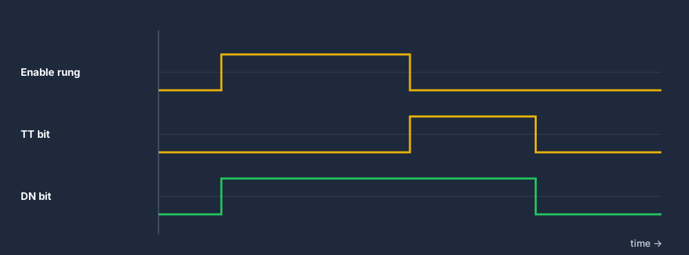
How it works. When the enable rung goes TRUE, EN and DN are set immediately — there is no delay on the leading edge. When the rung goes FALSE, EN clears, TT sets, and ACC begins counting. When ACC reaches PRE, TT clears and DN clears. If the rung goes TRUE again before ACC reaches PRE, ACC resets to zero and DN remains TRUE — the timer is retriggerable from the off-edge perspective.

A common point of confusion: the TOF done bit is TRUE during normal operation and only drops after the delay. This means you use the DN bit to keep equipment running, not to start it — the opposite polarity to how you use a TON.

TOF off-delay PLC timer timing diagram
TOF timing: DN is immediately TRUE when the rung energises, and stays TRUE for the full preset after the rung de-energises.

Real-world uses of the TOF timer

Fan run-on (motor cooling). After a motor stops, its windings retain heat. A cooling fan driven by a TOF keeps running for 60–300 seconds after the motor de-energises, preventing heat soak that shortens winding insulation life. The motor-run bit enables the TOF; the TOF DN bit keeps the fan on.

Door-seal alarm. A door-open sensor starts a TOF when the door closes. If the door opens again within the preset window, the timer resets — the system assumes the door is in normal use. Only if the door stays open past the preset does DN drop and trigger an alarm. This prevents nuisance alarms from brief access events.

Lubrication purge. After a conveyor stops, a lubrication pump continues running for a fixed period to flush debris from the lube lines. The TOF done bit keeps the pump on; when it drops, the pump stops.

Signal debounce on the falling edge. Where TON debounces the rising edge, TOF can debounce the falling edge — ignoring brief dropout events on a sensor that may flicker off momentarily during vibration. The DN bit stays TRUE through the flicker, only dropping if the sensor is consistently off for the preset duration.

Pulse timer

TP — pulse timer

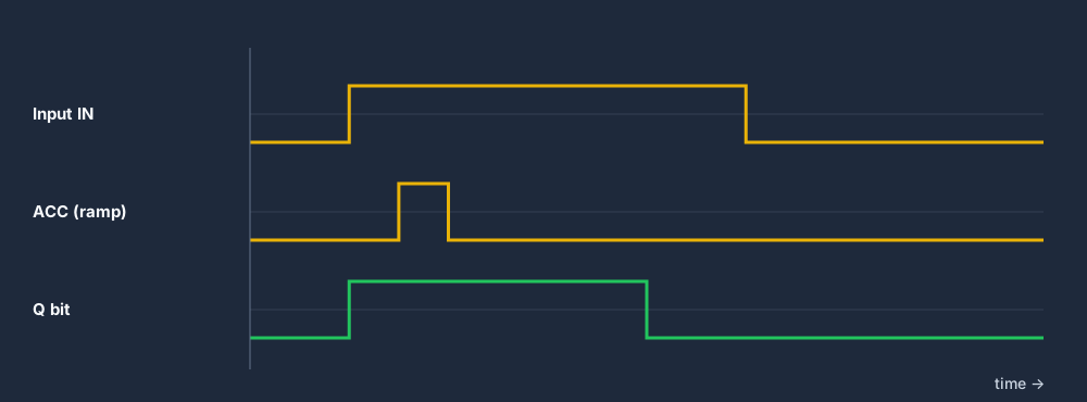
The TP (pulse) timer fires a fixed-duration output pulse on the rising edge of its enable input. Once triggered, the output Q remains TRUE for exactly the preset duration — it cannot be shortened by removing the input, and it cannot be extended by holding or re-applying the input during the pulse.

How it works. On a rising edge of the enable rung, Q is immediately set TRUE and ACC begins counting. The rung input is ignored until ACC reaches PT. When ACC reaches PT, Q is cleared and ACC resets — only at that point can a new rising edge retrigger the pulse. This non-retriggerable behaviour is the defining characteristic that separates TP from TON.

In Allen-Bradley ladder logic, TP is part of the IEC 61131-3 instruction set available in the Logix function block palette. Some legacy AB programs achieve the same result by combining a TON with a one-shot (OSR) contact, but the native TP instruction is cleaner and more readable.

TP pulse timer timing diagram PLC ladder logic
TP timing: Q fires for exactly PT on the rising edge. Removing or re-applying the input during the pulse has no effect — the pulse runs to completion.

How TP differs from TON

The critical difference is input control during timing. With a TON, dropping the input before PRE is reached cancels the timer and resets ACC. With a TP, the input is locked out during the pulse — the output runs for the full preset regardless. This makes TP better for:

  • Solenoid pulse actuation. Energising a solenoid for exactly 500 ms to actuate a cylinder, regardless of how long the operator holds the button.
  • Glue or paint gun burst. Dispensing a fixed volume of adhesive or paint on each part, triggered by a part-present sensor. The pulse length sets the dispense volume.
  • Single-shot alarm acknowledgement delay. After an alarm is acknowledged, disable re-acknowledgement for a fixed window to prevent accidental rapid acknowledgement of subsequent faults.
  • Heartbeat generation. A TP can generate a periodic pulse when combined with a self-resetting logic structure, though a dedicated clock bit is cleaner in practice.

Retentive on-delay timer

RTO / TONR — retentive on-delay timer

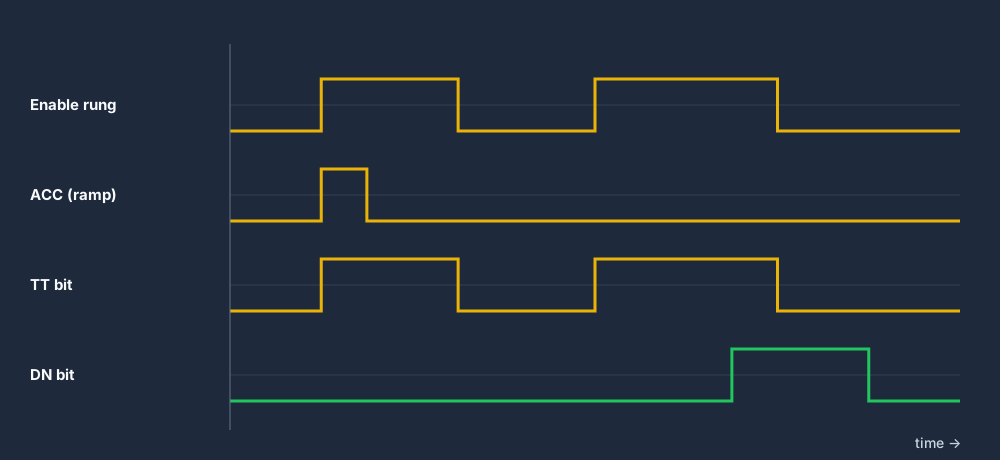
The RTO (retentive on-delay, also called TONR in IEC 61131-3) behaves like a TON in the forward direction — it counts while the rung is TRUE — but unlike a TON, it retains its accumulated value when the rung goes FALSE. The accumulator only resets when a dedicated RES (reset) instruction is explicitly triggered on a separate rung.

How it works. When the enable rung goes TRUE, EN is set, TT is set, and ACC increments. When the rung goes FALSE, EN and TT clear, but ACC holds its value. When the rung goes TRUE again, timing resumes from the held ACC value. When ACC finally reaches PRE, DN is set and TT clears. A separate RES rung — typically connected to a reset push-button or an automatic reset condition — clears ACC and DN, allowing the cycle to begin again.

This "memory across power loss" characteristic (on PLCs with battery-backed memory or retentive data) makes RTO suitable for long-term accumulation across multiple machine cycles or shift changes.

RTO retentive timer PLC timing diagram accumulator
RTO timing: ACC holds its value when the rung drops FALSE, resuming from the same point on the next TRUE edge. A RES instruction is required to reset.
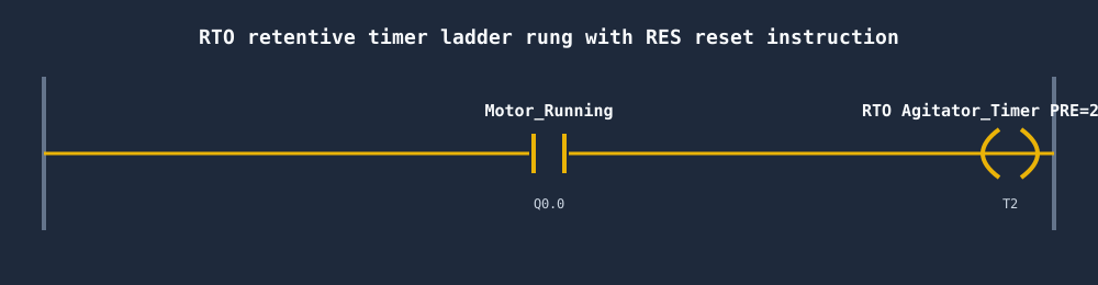
RTO retentive timer ladder rung with reset instruction
The RTO requires two rungs: one with the RTO instruction (enable) and a second with a RES instruction (reset) connected to a Reset push-button.

When to use RTO instead of TON

Use RTO whenever you need to accumulate runtime across interruptions. Common applications:

  • Motor run-time maintenance counter. Track total motor operating hours across all start/stop cycles since the last service. When ACC reaches PRE (e.g. 2,000 hours), a maintenance-required bit triggers a service reminder on the HMI.
  • Batch processing time. Accumulate total agitator run time across pauses for ingredient additions. The batch recipe requires exactly 45 minutes of mixing — even if the mix is paused for 10-minute ingredient loading steps.
  • Shift production timer. Accumulate actual production time within a shift, excluding planned downtime. The RES is triggered at shift end to reset for the next shift.
  • Filter service life. Count total airflow time through a filter. Reset at filter change. Trigger a change reminder when accumulated time exceeds the manufacturer's service interval.

The common thread: whenever the total accumulated time matters more than any single continuous run, choose RTO over TON.

Side-by-side

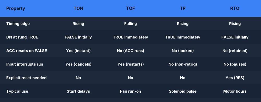
PLC timer types comparison: TON vs TOF vs TP vs RTO

The four standard PLC timer types differ on exactly three axes: which edge triggers timing, whether the accumulator is retained when the input drops, and whether the input can interrupt an in-progress timing cycle. For the two you will reach for most, see the full TON vs TOF breakdown with timing diagrams.

PLC timer types comparison TON TOF TP RTO
Comparison of TON, TOF, TP, and RTO across the key behavioural dimensions.

TON — On-delay

  • Delays the ON of the output
  • EN rung TRUE → ACC counts up
  • DN sets when ACC = PRE
  • ACC resets immediately when rung goes FALSE
  • Use for: motor start delays, debounce, alarm delays

TOF — Off-delay

  • Delays the OFF of the output
  • DN is TRUE immediately on enable
  • Timing starts when rung goes FALSE
  • DN drops when ACC = PRE after rung is FALSE
  • Use for: fan run-on, door alarms, purge cycles

TP — Pulse

  • Fixed-duration output pulse
  • Rising edge triggers; input locked during pulse
  • Q cannot be shortened or extended mid-pulse
  • ACC resets automatically at end of pulse
  • Use for: solenoid pulses, dispense bursts

RTO — Retentive on-delay

  • Accumulates time across interruptions
  • ACC holds value when rung goes FALSE
  • Requires an explicit RES rung to reset ACC
  • DN holds after preset reached until RES
  • Use for: motor hours, batch time, filter life
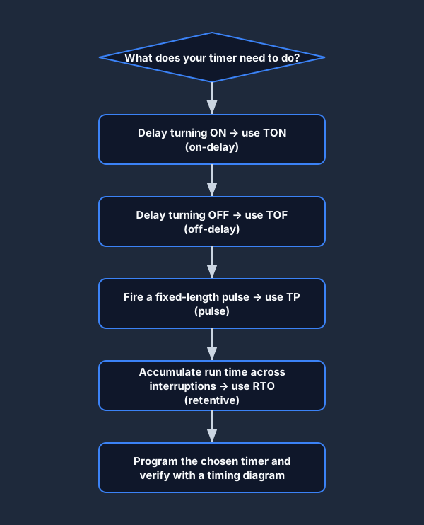
how to choose a PLC timer TON TOF TP RTO decision guide
Decision guide: start with this flowchart when choosing a timer type for a new application.

Naming conventions

Allen-Bradley vs IEC 61131-3 timer naming

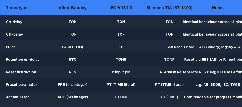
The PLC industry never standardised on a single instruction name for timers, so the same logical behaviour carries different mnemonics depending on your vendor. The IEC 61131-3 standard (published in 1993 and revised in 2013) attempted to unify naming, and modern platforms largely follow it — but Allen-Bradley's legacy naming from the RSLogix era remains widely used in North American industry.

The practical impact: if you can program a TON in Allen-Bradley, you can program a TON in Siemens TIA Portal, Codesys, OpenPLC, and Mitsubishi GX Works with nothing more than a naming lookup. The underlying scan-cycle logic, the preset/accumulator model, and the status bits are identical across vendors.

Allen Bradley IEC PLC timer names comparison table
Allen-Bradley and IEC 61131-3 timer instruction name mapping across major vendors.

Allen-Bradley (RSLogix / Studio 5000)

  • TON — on-delay timer. Parameters: PRE (ms), ACC (ms), bits: EN, TT, DN.
  • TOF — off-delay timer. Same parameters and bits as TON.
  • RTO — retentive on-delay. Same parameters; ACC survives rung FALSE; needs RES to reset.
  • RES — reset instruction. Used with RTO (and counters) to clear ACC and DN.
  • TP pulse timer is available via the IEC Function Block instructions in Studio 5000 Logix.

IEC 61131-3 (Siemens, Codesys, OpenPLC)

  • TON — on-delay. Parameters: IN (BOOL), PT (TIME); outputs: Q (BOOL), ET (TIME).
  • TOF — off-delay. Same interface as TON.
  • TP — pulse. Same interface; non-retriggerable fixed-duration pulse.
  • TONR — retentive on-delay (IEC equivalent of AB's RTO). Reset via R input pin.
  • Siemens uses IEC-compliant names in TIA Portal (S7-1200/1500). Older S7-300/400 used legacy S5 timer types (SD, SE, SS, SF, SP) — now deprecated.
Mitsubishi note. GX Works uses OUT T (output timer coil) with a K-value preset entered separately — e.g. LD X0 / OUT T1 K50 (T1, 5.0 seconds on a 100 ms timebase). Timer numbers determine the timebase: T0–T199 are 100 ms; T200–T245 are 10 ms on many FX series models. The concept is identical to IEC TON; only the syntax differs.

PLC timer programming examples

PLC timer programming examples

The following examples cover the four most common timer applications in industrial ladder logic. Each maps to a specific timer type and explains why that type is the right choice.

1. Conveyor start delay (TON)

A packaging conveyor must not start instantly when the operator presses Run. The downstream accumulation table needs 3 seconds to clear before the conveyor loads it with product. A TON with a 3,000 ms preset handles this cleanly.

Rung 1: XIC RunPB — XIC OL_OK — TON Conveyor_Start_Timer PRE=3000 ms
Rung 2: XIC Conveyor_Start_Timer.DN — OTE Conveyor_Motor

The Run push-button energises the TON. After 3 seconds of continuous Run input (operator did not release early), DN fires and the motor output energises. If the operator releases and re-presses before 3 seconds, ACC resets — the delay restarts. This is intentional: the full 3-second window must elapse from the last press.

2. Fan run-on after motor stop (TOF)

A motor-driven pump generates heat. A cooling fan must continue running for 90 seconds after the pump stops to prevent heat soak in the motor windings. A TOF on the motor-run bit provides this automatically.

Rung 1: XIC Pump_Motor — TOF Cooling_Fan_Timer PRE=90000 ms
Rung 2: XIC Cooling_Fan_Timer.DN — OTE Cooling_Fan

When Pump_Motor is TRUE, the TOF DN is immediately TRUE and the fan runs. When Pump_Motor goes FALSE, TOF begins timing. The fan continues running (DN stays TRUE) for 90 seconds, then DN drops and the fan stops. If the pump restarts within the 90-second window, ACC resets and DN stays TRUE — the fan never stopped, which is correct behaviour.

3. Alarm acknowledgement pulse (TP)

When an operator acknowledges an alarm, a one-second pulse should flash the panel acknowledge light and momentarily silence the horn. The pulse must be exactly one second regardless of how long the operator holds the acknowledge button.

Rung 1: XIC Ack_PB — TP Ack_Pulse_Timer PT=T#1S
Rung 2: XIC Ack_Pulse_Timer.Q — OTE Ack_Light
Rung 3: XIC Ack_Pulse_Timer.Q — OTE Horn_Silence

The TP fires on the rising edge of Ack_PB. For exactly one second, Q is TRUE, illuminating the light and silencing the horn. After one second, Q drops regardless of whether Ack_PB is still pressed. This prevents the operator from silencing alarms indefinitely by holding the button.

4. Batch agitator total run time (RTO)

A chemical batch process requires 45 minutes of agitation across a multi-step recipe. The agitator is paused for 5-minute ingredient loading steps three times during the batch. A TON would reset each time the agitator pauses — after 45 minutes of wall-clock time, only 30 minutes of actual agitation would have accumulated. An RTO solves this by retaining ACC through the pauses.

Rung 1: XIC Agitator_Running — RTO Agitator_Run_Timer PRE=2700000 ms (45 min)
Rung 2: XIC Agitator_Run_Timer.DN — OTE Batch_Mix_Complete
Rung 3: XIC Batch_Reset — RES Agitator_Run_Timer

ACC accumulates only while Agitator_Running is TRUE, holding its value during each pause. When the total reaches 2,700,000 ms, DN sets, triggering the batch-complete signal. Rung 3 resets everything at batch start or operator reset. This is the quintessential RTO application.

Live browser simulator

Try a live PLC timer — no install, no licence

Drop into a scenario, place a TON or TOF on a rung, set the preset, energise the input — and watch ACC count up in real time. The simulator grades your solution automatically.

Beginner

TON: Start Delay

Drop a TON on a rung, set a preset, and energise the input — watch ACC count toward DN.

Open scenario →
Curriculum

Curriculum: TON timer

A graded curriculum scenario building a motor start-delay circuit with a TON.

Open scenario →
Curriculum

Curriculum: TOF timer

Build a fan run-on circuit with a TOF off-delay timer. Auto-graded.

Open scenario →
Beginner

Conveyor Stop Delay

Use a TOF to keep a conveyor running for 5 seconds after the Stop signal arrives.

Open scenario →

Why a live simulator beats reading about timers

Watch ACC increment in real time — not just a static timing diagram
See exactly what happens when you drop the input before PRE is reached
Immediately observe the TOF "DN is already TRUE" behaviour that trips most beginners
Test retentive accumulation across multiple enable cycles with RTO
Get auto-graded feedback — know whether your timer logic is correct
Practice in Allen-Bradley dialect or switch to IEC 61131-3 names

Practice PLC timers free — in your browser.

Two auto-graded scenarios unlocked immediately. No credit card. No install. Works on Mac, Windows, Linux and Chromebook.

Questions

PLC timer FAQ

A TON (on-delay timer) starts counting when the rung goes TRUE and sets its DN/Q bit after the preset time elapses — DN drops immediately when the rung goes FALSE. A TOF (off-delay timer) works in reverse: DN is TRUE as long as the rung is energised, and the timer only starts counting when the rung goes FALSE. DN stays TRUE for the preset duration after the rung de-energises, then drops.

Watch a TON timer count in your browser today

No licence. No install. No credit card. Just ladder logic.

Create free account →

Technical reference and worked-example guide

PLC timer guide: implementation, evidence and troubleshooting

Direct answer

PLC timer guide becomes useful when it connects target platform, timer type, enabling condition, instance, time base, preset, elapsed value, status outputs, reset authority, task period, retentive state and restart with field condition through rung or code execution, timer state update, threshold comparison, downstream decision, physical result and independent elapsed measurement, then proves ton, tof and retentive examples each executed before, at and after preset from a known state under normal, boundary, fault and recovery conditions. The objective is a repeatable engineering or learning result, not merely activity inside a page or tool.

This guide is written for pLC learners and maintainers comparing delay-on, delay-off and retentive timing across scan cycles and vendor platforms. The intended result is specific: the reader can choose the timing contract, identify instance state and test exact preset, reset, dropout, restart and task-period boundaries.

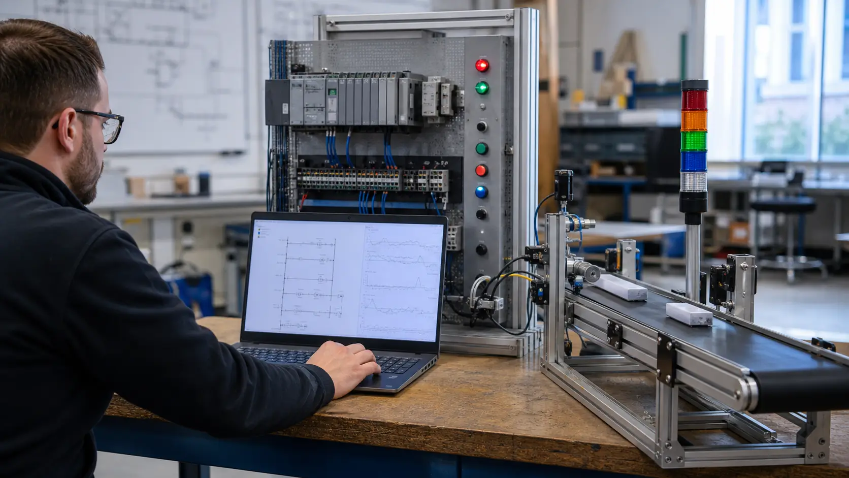
an automation engineer correlating PLC state, scan evidence and a controlled conveyor response at a logic diagnostics workstation while studying PLC TON, TOF and retentive timer selection and tests
The scene keeps PLC TON, TOF and retentive timer selection and tests connected to declared conditions, observable behavior, diagnostic boundaries and evidence that another person can reproduce.

System map / 02

Six concepts that control the result

Treat these as connected checkpoints. Each checkpoint has an expected state, an observable state and a boundary to the next part of the system. That structure prevents a software indication from being mistaken for physical proof.

NODE 01observable

Define the operating contract

target platform, timer type, enabling condition, instance, time base, preset, elapsed value, status outputs, reset authority, task period, retentive state and restart. For PLC TON, TOF and retentive timer selection and tests, record the initial condition, actor, requested change, observable result and stopping condition before selecting a tool or implementation.

NODE 02observable

Map the evidence path

field condition through rung or code execution, timer state update, threshold comparison, downstream decision, physical result and independent elapsed measurement. Separate request, internal state, output or service, physical or user-visible result and independent feedback so each boundary can be inspected.

NODE 03observable

Prove normal operation

TON, TOF and retentive examples each executed before, at and after preset from a known state. Run more than one cycle from a known state and retain the values, timings or artifacts that demonstrate repeatability.

NODE 04observable

Exercise a boundary case

brief input change, repeated call, skipped call, reset at preset, task jitter, maximum preset, overflow, mode change, download and power return. Choose minimum, maximum, simultaneous, delayed or restart conditions that reveal assumptions hidden by the happy path.

NODE 05observable

Diagnose a controlled fault

an instruction-type, enable, instance, time-base, scan, reset, retention, threshold, downstream-owner or restart mismatch. Preserve the first symptom, divide the system at a measurable boundary and change one condition only after predicting the result.

NODE 06observable

Transfer and hand over

the selected timer verified in current official target documentation and measured representative runtime tests. Restore normal state, remove temporary changes, repeat affected checks and document which claims remain limited to the learning environment.

Procedure / 03

A six-step practice and commissioning workflow

Run the steps in order the first time. Later, the same structure becomes a diagnostic loop: define the expected condition, observe the boundary, interpret the difference and choose one proving action.

  1. 01

    Write the acceptance case

    Convert target platform, timer type, enabling condition, instance, time base, preset, elapsed value, status outputs, reset authority, task period, retentive state and restart into initial conditions, one stimulus and observable pass criteria.

    Evidence: Another person can repeat the case without guessing the intended result.

    Avoid: Using page completion or an animation as the acceptance criterion.

  2. 02

    Build the map

    Document field condition through rung or code execution, timer state update, threshold comparison, downstream decision, physical result and independent elapsed measurement and name who owns each state or decision.

    Evidence: Every request and result has a source, destination and useful inspection point.

    Avoid: Using the same value as command, status and independent feedback.

  3. 03

    Run the baseline

    Apply ton, tof and retentive examples each executed before, at and after preset from a known state from a clean start and record the expected evidence.

    Evidence: Repeated runs produce the same bounded result.

    Avoid: Changing several parameters before a baseline exists.

  4. 04

    Challenge assumptions

    Test brief input change, repeated call, skipped call, reset at preset, task jitter, maximum preset, overflow, mode change, download and power return without changing the acceptance contract.

    Evidence: Limits, timing and restart behavior reach defined states.

    Avoid: Testing only one ideal sequence.

  5. 05

    Isolate one failure

    Introduce or analyse an instruction-type, enable, instance, time-base, scan, reset, retention, threshold, downstream-owner or restart mismatch and locate the first disagreement.

    Evidence: The proving action distinguishes the leading hypotheses.

    Avoid: Resetting, forcing or replacing before evidence is retained.

  6. 06

    Close the evidence loop

    Complete the selected timer verified in current official target documentation and measured representative runtime tests and repeat the affected regression cases.

    Evidence: Reference use is complete when inputs, assumptions, units or initial conditions are recorded and the result is independently checked at a useful boundary.

    Avoid: Treating an acknowledged message or one successful rerun as handover.

Diagnostic matrix / 04

Symptoms, proving points and next actions

The table is a reasoning aid, not a parts-replacement chart. Preserve the initial symptom, inspect the named boundary and use the interpretation to choose the next controlled test. Site safety procedures and equipment manuals remain authoritative.

Diagnostic symptoms, inspection points, interpretations and next actions for PLC timer guide: implementation, evidence and troubleshooting
Observed symptomInspectInterpretationNext proving action
The expected result is unclearRequirement, initial state, actor, stimulus, units and pass conditionThe technician, programmer and reviewer may be solving different versions of the task.Rewrite one observable acceptance case before continuing.
Internal state changes but the outcome does notRequest, final owner, output or service boundary and independent feedbackA software or interface indication proves intent at one layer, not the complete outcome.Trace the first boundary after the changing state.
Normal case passes but an edge case failsLimits, timing, simultaneous events, reset and restart assumptionsThe implementation contains a hidden assumption exposed by the changed condition.Add the failed boundary as a permanent regression case.
The failure disappears after resetOriginal symptom, histories, diagnostics, timestamps and active causeReset changed evidence or state without proving the initiating cause.Reproduce under a controlled condition and preserve pre/post-event data.
Simulator and target disagreeModel boundary, software version, task timing, I/O behavior, data types and configurationA learning model and the intended target do not share one of the recorded assumptions.Reduce the case and verify against current target documentation.
The result cannot be explainedPrediction, observation, proving action, alternative hypotheses and limitationsActivity occurred but the evidence is not yet transferable or reviewable.Have the learner defend the signal path and repeat a changed case.

Product evidence / 05

What the browser practice can actually demonstrate

The page connects definitions and worked examples to runnable tools, explicit assumptions and repeatable checks so a formula or pattern can be challenged.

Where simulation stops

Timer mnemonics are not semantic guarantees; target controller, time representation, task execution, call pattern and firmware determine exact behavior.

Commissioning notebook / 06

Six cases that turn the concepts into evidence

Use these as written briefs rather than click-through instructions. For every case, state the expected condition before acting, retain the first useful observation and explain why the final result proves the requirement. A different program or component choice can still be correct when it produces the same bounded behavior and evidence.

Case 01

predict → observe → prove

Prove define the operating contract

Engineering context. target platform, timer type, enabling condition, instance, time base, preset, elapsed value, status outputs, reset authority, task period, retentive state and restart. For PLC TON, TOF and retentive timer selection and tests, record the initial condition, actor, requested change, observable result and stopping condition before selecting a tool or implementation. Begin with a written normal condition and identify which request, state, physical result or communication value will provide independent confirmation. Do not begin by changing the configuration; the initial state is part of the evidence and should remain reproducible.

Controlled setup. Use the “Write the acceptance case” stage of the workflow: convert target platform, timer type, enabling condition, instance, time base, preset, elapsed value, status outputs, reset authority, task period, retentive state and restart into initial conditions, one stimulus and observable pass criteria. The acceptance record should show this result: another person can repeat the case without guessing the intended result. Record initial conditions, the exact stimulus and the observation point so another learner can repeat the case without relying on your memory.

Fault challenge. Introduce or analyse “The expected result is unclear” as one bounded deviation. Inspect requirement, initial state, actor, stimulus, units and pass condition The working interpretation is that the technician, programmer and reviewer may be solving different versions of the task. The next proving action is to rewrite one observable acceptance case before continuing. Change only one condition before observing the result, and preserve timestamps or measurements where timing matters.

Review and recovery. The most common trap here is using page completion or an animation as the acceptance criterion. After restoring the cause, repeat the normal case and at least one stop, timeout, disconnect or restart boundary relevant to this topic. Remove temporary forces and bypasses, return the model to a known state and retain the evidence that both operation and recovery are deliberate.

Explain it aloud: What are the main PLC timer types? A defensible short answer is: Common types include delay-on, delay-off and retentive on-delay behavior, but instruction names, stored state, outputs and reset rules vary by platform.

Case 02

predict → observe → prove

Prove map the evidence path

Engineering context. field condition through rung or code execution, timer state update, threshold comparison, downstream decision, physical result and independent elapsed measurement. Separate request, internal state, output or service, physical or user-visible result and independent feedback so each boundary can be inspected. Begin with a written normal condition and identify which request, state, physical result or communication value will provide independent confirmation. Do not begin by changing the configuration; the initial state is part of the evidence and should remain reproducible.

Controlled setup. Use the “Build the map” stage of the workflow: document field condition through rung or code execution, timer state update, threshold comparison, downstream decision, physical result and independent elapsed measurement and name who owns each state or decision. The acceptance record should show this result: every request and result has a source, destination and useful inspection point. Record initial conditions, the exact stimulus and the observation point so another learner can repeat the case without relying on your memory.

Fault challenge. Introduce or analyse “Internal state changes but the outcome does not” as one bounded deviation. Inspect request, final owner, output or service boundary and independent feedback The working interpretation is that a software or interface indication proves intent at one layer, not the complete outcome. The next proving action is to trace the first boundary after the changing state. Change only one condition before observing the result, and preserve timestamps or measurements where timing matters.

Review and recovery. The most common trap here is using the same value as command, status and independent feedback. After restoring the cause, repeat the normal case and at least one stop, timeout, disconnect or restart boundary relevant to this topic. Remove temporary forces and bypasses, return the model to a known state and retain the evidence that both operation and recovery are deliberate.

Explain it aloud: How accurate is a PLC timer? A defensible short answer is: Observed timing depends on task scheduling, scan period, instruction execution, time representation, I/O update and output latency; measure the complete required path.

Case 03

predict → observe → prove

Prove prove normal operation

Engineering context. TON, TOF and retentive examples each executed before, at and after preset from a known state. Run more than one cycle from a known state and retain the values, timings or artifacts that demonstrate repeatability. Begin with a written normal condition and identify which request, state, physical result or communication value will provide independent confirmation. Do not begin by changing the configuration; the initial state is part of the evidence and should remain reproducible.

Controlled setup. Use the “Run the baseline” stage of the workflow: apply ton, tof and retentive examples each executed before, at and after preset from a known state from a clean start and record the expected evidence. The acceptance record should show this result: repeated runs produce the same bounded result. Record initial conditions, the exact stimulus and the observation point so another learner can repeat the case without relying on your memory.

Fault challenge. Introduce or analyse “Normal case passes but an edge case fails” as one bounded deviation. Inspect limits, timing, simultaneous events, reset and restart assumptions The working interpretation is that the implementation contains a hidden assumption exposed by the changed condition. The next proving action is to add the failed boundary as a permanent regression case. Change only one condition before observing the result, and preserve timestamps or measurements where timing matters.

Review and recovery. The most common trap here is changing several parameters before a baseline exists. After restoring the cause, repeat the normal case and at least one stop, timeout, disconnect or restart boundary relevant to this topic. Remove temporary forces and bypasses, return the model to a known state and retain the evidence that both operation and recovery are deliberate.

Explain it aloud: What should I learn first about PLC TON, TOF and retentive timer selection and tests? A defensible short answer is: Start with the operating contract and evidence path: target platform, timer type, enabling condition, instance, time base, preset, elapsed value, status outputs, reset authority, task period, retentive state and restart, followed by field condition through rung or code execution, timer state update, threshold comparison, downstream decision, physical result and independent elapsed measurement. Add advanced features only after the baseline is predictable.

Case 04

predict → observe → prove

Prove exercise a boundary case

Engineering context. brief input change, repeated call, skipped call, reset at preset, task jitter, maximum preset, overflow, mode change, download and power return. Choose minimum, maximum, simultaneous, delayed or restart conditions that reveal assumptions hidden by the happy path. Begin with a written normal condition and identify which request, state, physical result or communication value will provide independent confirmation. Do not begin by changing the configuration; the initial state is part of the evidence and should remain reproducible.

Controlled setup. Use the “Challenge assumptions” stage of the workflow: test brief input change, repeated call, skipped call, reset at preset, task jitter, maximum preset, overflow, mode change, download and power return without changing the acceptance contract. The acceptance record should show this result: limits, timing and restart behavior reach defined states. Record initial conditions, the exact stimulus and the observation point so another learner can repeat the case without relying on your memory.

Fault challenge. Introduce or analyse “The failure disappears after reset” as one bounded deviation. Inspect original symptom, histories, diagnostics, timestamps and active cause The working interpretation is that reset changed evidence or state without proving the initiating cause. The next proving action is to reproduce under a controlled condition and preserve pre/post-event data. Change only one condition before observing the result, and preserve timestamps or measurements where timing matters.

Review and recovery. The most common trap here is testing only one ideal sequence. After restoring the cause, repeat the normal case and at least one stop, timeout, disconnect or restart boundary relevant to this topic. Remove temporary forces and bypasses, return the model to a known state and retain the evidence that both operation and recovery are deliberate.

Explain it aloud: How do I practise PLC TON, TOF and retentive timer selection and tests effectively? A defensible short answer is: Use short cases with known initial conditions, a written prediction, one action and an observable result. Then alter a boundary or fault and explain why the evidence changed.

Case 05

predict → observe → prove

Prove diagnose a controlled fault

Engineering context. an instruction-type, enable, instance, time-base, scan, reset, retention, threshold, downstream-owner or restart mismatch. Preserve the first symptom, divide the system at a measurable boundary and change one condition only after predicting the result. Begin with a written normal condition and identify which request, state, physical result or communication value will provide independent confirmation. Do not begin by changing the configuration; the initial state is part of the evidence and should remain reproducible.

Controlled setup. Use the “Isolate one failure” stage of the workflow: introduce or analyse an instruction-type, enable, instance, time-base, scan, reset, retention, threshold, downstream-owner or restart mismatch and locate the first disagreement. The acceptance record should show this result: the proving action distinguishes the leading hypotheses. Record initial conditions, the exact stimulus and the observation point so another learner can repeat the case without relying on your memory.

Fault challenge. Introduce or analyse “Simulator and target disagree” as one bounded deviation. Inspect model boundary, software version, task timing, I/O behavior, data types and configuration The working interpretation is that a learning model and the intended target do not share one of the recorded assumptions. The next proving action is to reduce the case and verify against current target documentation. Change only one condition before observing the result, and preserve timestamps or measurements where timing matters.

Review and recovery. The most common trap here is resetting, forcing or replacing before evidence is retained. After restoring the cause, repeat the normal case and at least one stop, timeout, disconnect or restart boundary relevant to this topic. Remove temporary forces and bypasses, return the model to a known state and retain the evidence that both operation and recovery are deliberate.

Explain it aloud: What counts as proof of competence? A defensible short answer is: A repeatable artifact or system result plus an explanation of the signal path is stronger than time spent, screenshots or a copied answer. Physical competence requires separate supervised evidence.

Case 06

predict → observe → prove

Prove transfer and hand over

Engineering context. the selected timer verified in current official target documentation and measured representative runtime tests. Restore normal state, remove temporary changes, repeat affected checks and document which claims remain limited to the learning environment. Begin with a written normal condition and identify which request, state, physical result or communication value will provide independent confirmation. Do not begin by changing the configuration; the initial state is part of the evidence and should remain reproducible.

Controlled setup. Use the “Close the evidence loop” stage of the workflow: complete the selected timer verified in current official target documentation and measured representative runtime tests and repeat the affected regression cases. The acceptance record should show this result: reference use is complete when inputs, assumptions, units or initial conditions are recorded and the result is independently checked at a useful boundary. Record initial conditions, the exact stimulus and the observation point so another learner can repeat the case without relying on your memory.

Fault challenge. Introduce or analyse “The result cannot be explained” as one bounded deviation. Inspect prediction, observation, proving action, alternative hypotheses and limitations The working interpretation is that activity occurred but the evidence is not yet transferable or reviewable. The next proving action is to have the learner defend the signal path and repeat a changed case. Change only one condition before observing the result, and preserve timestamps or measurements where timing matters.

Review and recovery. The most common trap here is treating an acknowledged message or one successful rerun as handover. After restoring the cause, repeat the normal case and at least one stop, timeout, disconnect or restart boundary relevant to this topic. Remove temporary forces and bypasses, return the model to a known state and retain the evidence that both operation and recovery are deliberate.

Explain it aloud: Why test faults and restart behavior? A defensible short answer is: Because an instruction-type, enable, instance, time-base, scan, reset, retention, threshold, downstream-owner or restart mismatch or brief input change, repeated call, skipped call, reset at preset, task jitter, maximum preset, overflow, mode change, download and power return can expose assumptions that never appear during ideal startup and steady operation.

Answer surface / 07

Questions people ask about PLC timer guide

These concise answers define the operating, training and product boundaries most often missed in broad summaries. The full workflow and diagnostic table above provide the evidence behind them.

What are the main PLC timer types?

Common types include delay-on, delay-off and retentive on-delay behavior, but instruction names, stored state, outputs and reset rules vary by platform.

How accurate is a PLC timer?

Observed timing depends on task scheduling, scan period, instruction execution, time representation, I/O update and output latency; measure the complete required path.

What should I learn first about PLC TON, TOF and retentive timer selection and tests?

Start with the operating contract and evidence path: target platform, timer type, enabling condition, instance, time base, preset, elapsed value, status outputs, reset authority, task period, retentive state and restart, followed by field condition through rung or code execution, timer state update, threshold comparison, downstream decision, physical result and independent elapsed measurement. Add advanced features only after the baseline is predictable.

How do I practise PLC TON, TOF and retentive timer selection and tests effectively?

Use short cases with known initial conditions, a written prediction, one action and an observable result. Then alter a boundary or fault and explain why the evidence changed.

What counts as proof of competence?

A repeatable artifact or system result plus an explanation of the signal path is stronger than time spent, screenshots or a copied answer. Physical competence requires separate supervised evidence.

Why test faults and restart behavior?

Because an instruction-type, enable, instance, time-base, scan, reset, retention, threshold, downstream-owner or restart mismatch or brief input change, repeated call, skipped call, reset at preset, task jitter, maximum preset, overflow, mode change, download and power return can expose assumptions that never appear during ideal startup and steady operation.

Can browser practice replace official software or hardware?

No. It can build concepts and diagnostic reasoning. Exact firmware, I/O electrical behavior, networking, safety and commissioning require current official tools, documentation and target equipment.

How should progress be documented?

Keep the requirement, initial state, program or configuration, observed values, fault hypothesis, proving action, recovery result and a concise limitations statement.