← Back to all lessons
Wiring 11
Pro

Wiring 11 — Quadrature Encoder to PLC High-Speed Counter Input

What you'll learn

An incremental quadrature encoder produces two digital pulse trains — A and B — that are 90° out of phase with each other. Because of this phase offset, the PLC can determine both position (by counting edges) and direction of travel: when A leads B the axis is moving forward; when B leads A the axis is moving in reverse. A third signal, Z, produces a single pulse per revolution at a repeatable mechanical position. This index or marker pulse is used to establish an absolute reference after a power cycle or alarm recovery — without it the PLC only ever knows relative displacement from wherever it started.

Lab time: ~18 minutes.

Lesson briefing

Quadrature Encoder to PLC High-Speed Counter Input

The Quadrature Principle

An incremental quadrature encoder produces two digital pulse trains — A and B — that are 90° out of phase with each other. Because of this phase offset, the PLC can determine both position (by counting edges) and direction of travel: when A leads B the axis is moving forward; when B leads A the axis is moving in reverse. A third signal, Z, produces a single pulse per revolution at a repeatable mechanical position. This index or marker pulse is used to establish an absolute reference after a power cycle or alarm recovery — without it the PLC only ever knows relative displacement from wherever it started.

Why Line-Driver / Differential Wiring

Encoders are available in two output circuit types. Open-collector encoders use three signal wires (A, B, Z), a supply, a common, and a shield — six conductors total. They are cheap and adequate for cable runs up to roughly 5–10 metres.

In an industrial cabinet sharing cable trays with VFDs, contactors, and power wiring, open-collector signals are unacceptably noisy over longer runs. Line-driver (RS-422 differential) encoders solve this by sending each phase as a complementary pair: A and A' are always opposite in polarity. The HSC card's receiver subtracts A' from A; any noise that appears equally on both wires — called common-mode noise — cancels out mathematically. This is the same noise-rejection principle used by analog 4–20 mA loops and RS-485 networks. Line-driver wiring is the industrial default whenever cable runs exceed a few metres or EMI sources are present.

5V TTL vs 24V HTL Encoders

Line-driver encoders come in two voltage families. 5V TTL encoders are the traditional choice: they support higher pulse rates (up to several MHz), are cheaper, and suit servo drives with built-in 5V encoder supplies. 24V HTL encoders swing the signal rails to the full 24V bus, making them more immune to resistive voltage drop over long cable runs and compatible with standard PLC I/O supply rails. This lesson uses a 24V encoder — the more common choice in general-purpose industrial automation.

Shield Grounding — One End Only

The encoder cable shield must be bonded to protective earth at exactly one point. In this topology, the shield bonds at the PLC HSC card's SHIELD terminal, which is internally connected to the cabinet ground bar. The encoder end of the shield is left floating. Bonding both ends creates a low-impedance loop between two ground points; any difference in earth potential between the machine frame and the control cabinet drives a circulating current through that loop, inducing noise directly on the differential signal — the exact problem you are trying to prevent. This single-point shield rule is identical to the rule you applied in lessons 06 and 07 for analog signals.

HSC Card vs General Digital Input

General-purpose DI cards can read encoder A and B signals at low speeds, but they route pulses through the PLC backplane and firmware scan cycle. Above a few kHz the firmware cannot keep up and pulses are lost. HSC cards contain dedicated quadrature decode logic in hardware (typically an FPGA counter): they latch every edge in real time, maintain a 32-bit position register, and detect direction without consuming any CPU scan time. Use an HSC card whenever an encoder operates above 1–2 kHz or when direction information is required with guaranteed accuracy.

Hints

Hint 1

Differential pairs travel together: wire A and A' as a matched pair to HSC-A and HSC-A', then B and B' to HSC-B and HSC-B', then Z and Z' to HSC-Z and HSC-Z'. Never wire a true output to the complement input or vice versa — the direction logic will invert.

Hint 2

Sign up to unlock the full hint sequence.

Hint 3

Sign up to unlock the full hint sequence.

Hint 4

Sign up to unlock the full hint sequence.

Hint 5

Sign up to unlock the full hint sequence.

This lesson uses 8 placed components on the lab canvas. Components are vendor-neutral (no proprietary trademarks); the wiring rules apply to any equivalent industrial part.

Sign up to preview

Create a free account to preview this Pro lab; upgrade to open the interactive circuit.

Sign up to preview

You might also like

Competency and practice field guide

Quadrature-encoder PLC wiring lesson: implementation, evidence and troubleshooting

Direct answer

Quadrature-encoder PLC wiring lesson becomes useful when it connects encoder supply, output driver, common reference, a and b channels, index, complementary outputs, cable, shield, input type, count frequency, resolution and mechanics with shaft motion through optical or magnetic edges, channel phase, conductor path, high-speed input, count and direction logic, scaled position and independent motion evidence, then proves forward and reverse motion produce the expected phase order, count sign and repeatable scaled displacement under normal, boundary, fault and recovery conditions. The objective is a repeatable engineering or learning result, not merely activity inside a page or tool.

This guide is written for pLC and electrical learners connecting encoder power, common, A and B channels, optional index and high-speed inputs. The intended result is specific: the learner can predict phase order and count direction, verify electrical compatibility and distinguish wiring, speed, configuration and scaling faults.

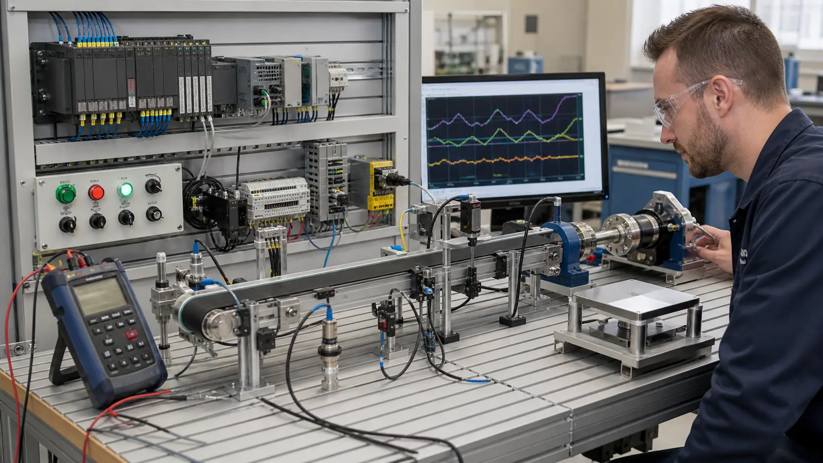
a technician tracing realistic industrial sensors, signal wiring, PLC inputs and measured trends at an instrumentation learning bench while studying A/B quadrature encoder wiring, direction and count evidence
The scene keeps A/B quadrature encoder wiring, direction and count evidence connected to declared conditions, observable behavior, diagnostic boundaries and evidence that another person can reproduce.

System map / 02

Six concepts that control the result

Treat these as connected checkpoints. Each checkpoint has an expected state, an observable state and a boundary to the next part of the system. That structure prevents a software indication from being mistaken for physical proof.

NODE 01observable

Define the operating contract

encoder supply, output driver, common reference, A and B channels, index, complementary outputs, cable, shield, input type, count frequency, resolution and mechanics. For A/B quadrature encoder wiring, direction and count evidence, record the initial condition, actor, requested change, observable result and stopping condition before selecting a tool or implementation.

NODE 02observable

Map the evidence path

shaft motion through optical or magnetic edges, channel phase, conductor path, high-speed input, count and direction logic, scaled position and independent motion evidence. Separate request, internal state, output or service, physical or user-visible result and independent feedback so each boundary can be inspected.

NODE 03observable

Prove normal operation

forward and reverse motion produce the expected phase order, count sign and repeatable scaled displacement. Run more than one cycle from a known state and retain the values, timings or artifacts that demonstrate repeatability.

NODE 04observable

Exercise a boundary case

reversed channels, missing common, single lost channel, bounce or noise, excessive frequency, missed index, rollover, stopped jitter and power return. Choose minimum, maximum, simultaneous, delayed or restart conditions that reveal assumptions hidden by the happy path.

NODE 05observable

Diagnose a controlled fault

a mechanical, sensor, supply, interface, conductor, channel, input-configuration, frequency, count or scaling mismatch. Preserve the first symptom, divide the system at a measurable boundary and change one condition only after predicting the result.

NODE 06observable

Transfer and hand over

the full chain verified with actual encoder data, target high-speed input and measured representative motion. Restore normal state, remove temporary changes, repeat affected checks and document which claims remain limited to the learning environment.

Procedure / 03

A six-step practice and commissioning workflow

Run the steps in order the first time. Later, the same structure becomes a diagnostic loop: define the expected condition, observe the boundary, interpret the difference and choose one proving action.

  1. 01

    Write the acceptance case

    Convert encoder supply, output driver, common reference, a and b channels, index, complementary outputs, cable, shield, input type, count frequency, resolution and mechanics into initial conditions, one stimulus and observable pass criteria.

    Evidence: Another person can repeat the case without guessing the intended result.

    Avoid: Using page completion or an animation as the acceptance criterion.

  2. 02

    Build the map

    Document shaft motion through optical or magnetic edges, channel phase, conductor path, high-speed input, count and direction logic, scaled position and independent motion evidence and name who owns each state or decision.

    Evidence: Every request and result has a source, destination and useful inspection point.

    Avoid: Using the same value as command, status and independent feedback.

  3. 03

    Run the baseline

    Apply forward and reverse motion produce the expected phase order, count sign and repeatable scaled displacement from a clean start and record the expected evidence.

    Evidence: Repeated runs produce the same bounded result.

    Avoid: Changing several parameters before a baseline exists.

  4. 04

    Challenge assumptions

    Test reversed channels, missing common, single lost channel, bounce or noise, excessive frequency, missed index, rollover, stopped jitter and power return without changing the acceptance contract.

    Evidence: Limits, timing and restart behavior reach defined states.

    Avoid: Testing only one ideal sequence.

  5. 05

    Isolate one failure

    Introduce or analyse a mechanical, sensor, supply, interface, conductor, channel, input-configuration, frequency, count or scaling mismatch and locate the first disagreement.

    Evidence: The proving action distinguishes the leading hypotheses.

    Avoid: Resetting, forcing or replacing before evidence is retained.

  6. 06

    Close the evidence loop

    Complete the full chain verified with actual encoder data, target high-speed input and measured representative motion and repeat the affected regression cases.

    Evidence: A learner completes the surface by explaining the result, passing a changed case and identifying what still requires supervised target-equipment practice.

    Avoid: Treating an acknowledged message or one successful rerun as handover.

Diagnostic matrix / 04

Symptoms, proving points and next actions

The table is a reasoning aid, not a parts-replacement chart. Preserve the initial symptom, inspect the named boundary and use the interpretation to choose the next controlled test. Site safety procedures and equipment manuals remain authoritative.

Diagnostic symptoms, inspection points, interpretations and next actions for Quadrature-encoder PLC wiring lesson: implementation, evidence and troubleshooting
Observed symptomInspectInterpretationNext proving action
The expected result is unclearRequirement, initial state, actor, stimulus, units and pass conditionThe learner, instructor and assessor may be solving different versions of the task.Rewrite one observable acceptance case before continuing.
Internal state changes but the outcome does notRequest, final owner, output or service boundary and independent feedbackA software or interface indication proves intent at one layer, not the complete outcome.Trace the first boundary after the changing state.
Normal case passes but an edge case failsLimits, timing, simultaneous events, reset and restart assumptionsThe implementation contains a hidden assumption exposed by the changed condition.Add the failed boundary as a permanent regression case.
The failure disappears after resetOriginal symptom, histories, diagnostics, timestamps and active causeReset changed evidence or state without proving the initiating cause.Reproduce under a controlled condition and preserve pre/post-event data.
Simulator and target disagreeModel boundary, software version, task timing, I/O behavior, data types and configurationA learning model and the intended target do not share one of the recorded assumptions.Reduce the case and verify against current target documentation.
The result cannot be explainedPrediction, observation, proving action, alternative hypotheses and limitationsActivity occurred but the evidence is not yet transferable or reviewable.Have the learner defend the signal path and repeat a changed case.

Product evidence / 05

What the browser practice can actually demonstrate

The browser platform can retain programs, scenario results, attempts and observable machine state so practice is attached to evidence rather than seat time alone.

Where simulation stops

Virtual wiring cannot approve real encoder shielding, grounding, hazardous-area use, motion safety or controller high-speed capability.

Commissioning notebook / 06

Six cases that turn the concepts into evidence

Use these as written briefs rather than click-through instructions. For every case, state the expected condition before acting, retain the first useful observation and explain why the final result proves the requirement. A different program or component choice can still be correct when it produces the same bounded behavior and evidence.

Case 01

predict → observe → prove

Prove define the operating contract

Engineering context. encoder supply, output driver, common reference, A and B channels, index, complementary outputs, cable, shield, input type, count frequency, resolution and mechanics. For A/B quadrature encoder wiring, direction and count evidence, record the initial condition, actor, requested change, observable result and stopping condition before selecting a tool or implementation. Begin with a written normal condition and identify which request, state, physical result or communication value will provide independent confirmation. Do not begin by changing the configuration; the initial state is part of the evidence and should remain reproducible.

Controlled setup. Use the “Write the acceptance case” stage of the workflow: convert encoder supply, output driver, common reference, a and b channels, index, complementary outputs, cable, shield, input type, count frequency, resolution and mechanics into initial conditions, one stimulus and observable pass criteria. The acceptance record should show this result: another person can repeat the case without guessing the intended result. Record initial conditions, the exact stimulus and the observation point so another learner can repeat the case without relying on your memory.

Fault challenge. Introduce or analyse “The expected result is unclear” as one bounded deviation. Inspect requirement, initial state, actor, stimulus, units and pass condition The working interpretation is that the learner, instructor and assessor may be solving different versions of the task. The next proving action is to rewrite one observable acceptance case before continuing. Change only one condition before observing the result, and preserve timestamps or measurements where timing matters.

Review and recovery. The most common trap here is using page completion or an animation as the acceptance criterion. After restoring the cause, repeat the normal case and at least one stop, timeout, disconnect or restart boundary relevant to this topic. Remove temporary forces and bypasses, return the model to a known state and retain the evidence that both operation and recovery are deliberate.

Explain it aloud: What are encoder A and B channels? A defensible short answer is: They are pulse trains offset in phase; their transition order lets a compatible counter determine direction while the edge count represents motion.

Case 02

predict → observe → prove

Prove map the evidence path

Engineering context. shaft motion through optical or magnetic edges, channel phase, conductor path, high-speed input, count and direction logic, scaled position and independent motion evidence. Separate request, internal state, output or service, physical or user-visible result and independent feedback so each boundary can be inspected. Begin with a written normal condition and identify which request, state, physical result or communication value will provide independent confirmation. Do not begin by changing the configuration; the initial state is part of the evidence and should remain reproducible.

Controlled setup. Use the “Build the map” stage of the workflow: document shaft motion through optical or magnetic edges, channel phase, conductor path, high-speed input, count and direction logic, scaled position and independent motion evidence and name who owns each state or decision. The acceptance record should show this result: every request and result has a source, destination and useful inspection point. Record initial conditions, the exact stimulus and the observation point so another learner can repeat the case without relying on your memory.

Fault challenge. Introduce or analyse “Internal state changes but the outcome does not” as one bounded deviation. Inspect request, final owner, output or service boundary and independent feedback The working interpretation is that a software or interface indication proves intent at one layer, not the complete outcome. The next proving action is to trace the first boundary after the changing state. Change only one condition before observing the result, and preserve timestamps or measurements where timing matters.

Review and recovery. The most common trap here is using the same value as command, status and independent feedback. After restoring the cause, repeat the normal case and at least one stop, timeout, disconnect or restart boundary relevant to this topic. Remove temporary forces and bypasses, return the model to a known state and retain the evidence that both operation and recovery are deliberate.

Explain it aloud: What happens if A and B are swapped? A defensible short answer is: The indicated direction normally reverses, but exact behavior depends on counter mode and configuration; verify with controlled motion.

Case 03

predict → observe → prove

Prove prove normal operation

Engineering context. forward and reverse motion produce the expected phase order, count sign and repeatable scaled displacement. Run more than one cycle from a known state and retain the values, timings or artifacts that demonstrate repeatability. Begin with a written normal condition and identify which request, state, physical result or communication value will provide independent confirmation. Do not begin by changing the configuration; the initial state is part of the evidence and should remain reproducible.

Controlled setup. Use the “Run the baseline” stage of the workflow: apply forward and reverse motion produce the expected phase order, count sign and repeatable scaled displacement from a clean start and record the expected evidence. The acceptance record should show this result: repeated runs produce the same bounded result. Record initial conditions, the exact stimulus and the observation point so another learner can repeat the case without relying on your memory.

Fault challenge. Introduce or analyse “Normal case passes but an edge case fails” as one bounded deviation. Inspect limits, timing, simultaneous events, reset and restart assumptions The working interpretation is that the implementation contains a hidden assumption exposed by the changed condition. The next proving action is to add the failed boundary as a permanent regression case. Change only one condition before observing the result, and preserve timestamps or measurements where timing matters.

Review and recovery. The most common trap here is changing several parameters before a baseline exists. After restoring the cause, repeat the normal case and at least one stop, timeout, disconnect or restart boundary relevant to this topic. Remove temporary forces and bypasses, return the model to a known state and retain the evidence that both operation and recovery are deliberate.

Explain it aloud: What should I learn first about A/B quadrature encoder wiring, direction and count evidence? A defensible short answer is: Start with the operating contract and evidence path: encoder supply, output driver, common reference, a and b channels, index, complementary outputs, cable, shield, input type, count frequency, resolution and mechanics, followed by shaft motion through optical or magnetic edges, channel phase, conductor path, high-speed input, count and direction logic, scaled position and independent motion evidence. Add advanced features only after the baseline is predictable.

Case 04

predict → observe → prove

Prove exercise a boundary case

Engineering context. reversed channels, missing common, single lost channel, bounce or noise, excessive frequency, missed index, rollover, stopped jitter and power return. Choose minimum, maximum, simultaneous, delayed or restart conditions that reveal assumptions hidden by the happy path. Begin with a written normal condition and identify which request, state, physical result or communication value will provide independent confirmation. Do not begin by changing the configuration; the initial state is part of the evidence and should remain reproducible.

Controlled setup. Use the “Challenge assumptions” stage of the workflow: test reversed channels, missing common, single lost channel, bounce or noise, excessive frequency, missed index, rollover, stopped jitter and power return without changing the acceptance contract. The acceptance record should show this result: limits, timing and restart behavior reach defined states. Record initial conditions, the exact stimulus and the observation point so another learner can repeat the case without relying on your memory.

Fault challenge. Introduce or analyse “The failure disappears after reset” as one bounded deviation. Inspect original symptom, histories, diagnostics, timestamps and active cause The working interpretation is that reset changed evidence or state without proving the initiating cause. The next proving action is to reproduce under a controlled condition and preserve pre/post-event data. Change only one condition before observing the result, and preserve timestamps or measurements where timing matters.

Review and recovery. The most common trap here is testing only one ideal sequence. After restoring the cause, repeat the normal case and at least one stop, timeout, disconnect or restart boundary relevant to this topic. Remove temporary forces and bypasses, return the model to a known state and retain the evidence that both operation and recovery are deliberate.

Explain it aloud: How do I practise A/B quadrature encoder wiring, direction and count evidence effectively? A defensible short answer is: Use short cases with known initial conditions, a written prediction, one action and an observable result. Then alter a boundary or fault and explain why the evidence changed.

Case 05

predict → observe → prove

Prove diagnose a controlled fault

Engineering context. a mechanical, sensor, supply, interface, conductor, channel, input-configuration, frequency, count or scaling mismatch. Preserve the first symptom, divide the system at a measurable boundary and change one condition only after predicting the result. Begin with a written normal condition and identify which request, state, physical result or communication value will provide independent confirmation. Do not begin by changing the configuration; the initial state is part of the evidence and should remain reproducible.

Controlled setup. Use the “Isolate one failure” stage of the workflow: introduce or analyse a mechanical, sensor, supply, interface, conductor, channel, input-configuration, frequency, count or scaling mismatch and locate the first disagreement. The acceptance record should show this result: the proving action distinguishes the leading hypotheses. Record initial conditions, the exact stimulus and the observation point so another learner can repeat the case without relying on your memory.

Fault challenge. Introduce or analyse “Simulator and target disagree” as one bounded deviation. Inspect model boundary, software version, task timing, I/O behavior, data types and configuration The working interpretation is that a learning model and the intended target do not share one of the recorded assumptions. The next proving action is to reduce the case and verify against current target documentation. Change only one condition before observing the result, and preserve timestamps or measurements where timing matters.

Review and recovery. The most common trap here is resetting, forcing or replacing before evidence is retained. After restoring the cause, repeat the normal case and at least one stop, timeout, disconnect or restart boundary relevant to this topic. Remove temporary forces and bypasses, return the model to a known state and retain the evidence that both operation and recovery are deliberate.

Explain it aloud: What counts as proof of competence? A defensible short answer is: A repeatable artifact or system result plus an explanation of the signal path is stronger than time spent, screenshots or a copied answer. Physical competence requires separate supervised evidence.

Case 06

predict → observe → prove

Prove transfer and hand over

Engineering context. the full chain verified with actual encoder data, target high-speed input and measured representative motion. Restore normal state, remove temporary changes, repeat affected checks and document which claims remain limited to the learning environment. Begin with a written normal condition and identify which request, state, physical result or communication value will provide independent confirmation. Do not begin by changing the configuration; the initial state is part of the evidence and should remain reproducible.

Controlled setup. Use the “Close the evidence loop” stage of the workflow: complete the full chain verified with actual encoder data, target high-speed input and measured representative motion and repeat the affected regression cases. The acceptance record should show this result: a learner completes the surface by explaining the result, passing a changed case and identifying what still requires supervised target-equipment practice. Record initial conditions, the exact stimulus and the observation point so another learner can repeat the case without relying on your memory.

Fault challenge. Introduce or analyse “The result cannot be explained” as one bounded deviation. Inspect prediction, observation, proving action, alternative hypotheses and limitations The working interpretation is that activity occurred but the evidence is not yet transferable or reviewable. The next proving action is to have the learner defend the signal path and repeat a changed case. Change only one condition before observing the result, and preserve timestamps or measurements where timing matters.

Review and recovery. The most common trap here is treating an acknowledged message or one successful rerun as handover. After restoring the cause, repeat the normal case and at least one stop, timeout, disconnect or restart boundary relevant to this topic. Remove temporary forces and bypasses, return the model to a known state and retain the evidence that both operation and recovery are deliberate.

Explain it aloud: Why test faults and restart behavior? A defensible short answer is: Because a mechanical, sensor, supply, interface, conductor, channel, input-configuration, frequency, count or scaling mismatch or reversed channels, missing common, single lost channel, bounce or noise, excessive frequency, missed index, rollover, stopped jitter and power return can expose assumptions that never appear during ideal startup and steady operation.
Answer surface / 07

Questions people ask about Quadrature-encoder PLC wiring lesson

These concise answers define the operating, training and product boundaries most often missed in broad summaries. The full workflow and diagnostic table above provide the evidence behind them.

What are encoder A and B channels?

They are pulse trains offset in phase; their transition order lets a compatible counter determine direction while the edge count represents motion.

What happens if A and B are swapped?

The indicated direction normally reverses, but exact behavior depends on counter mode and configuration; verify with controlled motion.

What should I learn first about A/B quadrature encoder wiring, direction and count evidence?

Start with the operating contract and evidence path: encoder supply, output driver, common reference, a and b channels, index, complementary outputs, cable, shield, input type, count frequency, resolution and mechanics, followed by shaft motion through optical or magnetic edges, channel phase, conductor path, high-speed input, count and direction logic, scaled position and independent motion evidence. Add advanced features only after the baseline is predictable.

How do I practise A/B quadrature encoder wiring, direction and count evidence effectively?

Use short cases with known initial conditions, a written prediction, one action and an observable result. Then alter a boundary or fault and explain why the evidence changed.

What counts as proof of competence?

A repeatable artifact or system result plus an explanation of the signal path is stronger than time spent, screenshots or a copied answer. Physical competence requires separate supervised evidence.

Why test faults and restart behavior?

Because a mechanical, sensor, supply, interface, conductor, channel, input-configuration, frequency, count or scaling mismatch or reversed channels, missing common, single lost channel, bounce or noise, excessive frequency, missed index, rollover, stopped jitter and power return can expose assumptions that never appear during ideal startup and steady operation.

Can browser practice replace official software or hardware?

No. It can build concepts and diagnostic reasoning. Exact firmware, I/O electrical behavior, networking, safety and commissioning require current official tools, documentation and target equipment.

How should progress be documented?

Keep the requirement, initial state, program or configuration, observed values, fault hypothesis, proving action, recovery result and a concise limitations statement.